This lab journal replicates the analyses for ‘ceasing to publish’.

Custom functions

package.check: Check if packages are installed (and install if not) in R (source).

fpackage.check <- function(packages) {
  lapply(packages, FUN = function(x) {
    if (!require(x, character.only = TRUE)) {
      install.packages(x, dependencies = TRUE)
      library(x, character.only = TRUE)
    }
  })
}

fsave <- function(x, file, location="./data/processed/") {
  datename <- substr(gsub("[:-]", "", Sys.time()), 1,8)  
  totalname <- paste(location, datename, file, sep="")
  save(x, file = totalname)  
}

Packages

survival: general package to create life tables and survival models, needed for flexsurv
flexsurv: fitting flexible survival regression models
boot: bootstrapping for SEs of AMEs
tidyverse: for data manipulation
ggplot2: for creating figures 5-7
ggpubr: for combining two figures in one (plot 5)
kableExtra: formatting tables

packages = c("survival", "flexsurv", "boot", "tidyverse", "ggplot2", "ggpubr", "kableExtra") 

fpackage.check(packages)

## Loading required package: survival

## Loading required package: flexsurv

## Loading required package: boot

## 
## Attaching package: 'boot'

## The following object is masked from 'package:survival':
## 
##     aml

## Loading required package: kableExtra

## 
## Attaching package: 'kableExtra'

## The following object is masked from 'package:dplyr':
## 
##     group_rows

Input

We use two processed datasets.

df_stopping.rda: person-period file containing publications and all relevant variables for the survival models, time window for inactivity is 3 years
- For construction of this dataset see Dependent Variables : Starting and Stopping to Publish
- name of dataset: df_ppf3
df_stopping5.rda: person-period file containing publications and all relevant variables for the survival models, time-window for inactivity is years
- For construction of this dataset see Dependent Variables : Starting and Stopping to Publish
- name of dataset: df_ppf5

load(file = "./data/processed/df_stopping.rda")


load(file = "data/processed/df_stopping5.rda")

Checking distributions

Kaplan-Meier curve

KM1 <- survfit(Surv(time-1, time, inactive) ~ 1, conf.lower='usual', data = df_ppf3)
KM2 <- survfit(Surv(time-1, time, inactive) ~ gender, conf.lower='usual', data = df_ppf3)
KM3 <- survfit(Surv(time-1, time, inactive) ~ ethnicity2, conf.lower='usual', data = df_ppf3)


plot(KM1)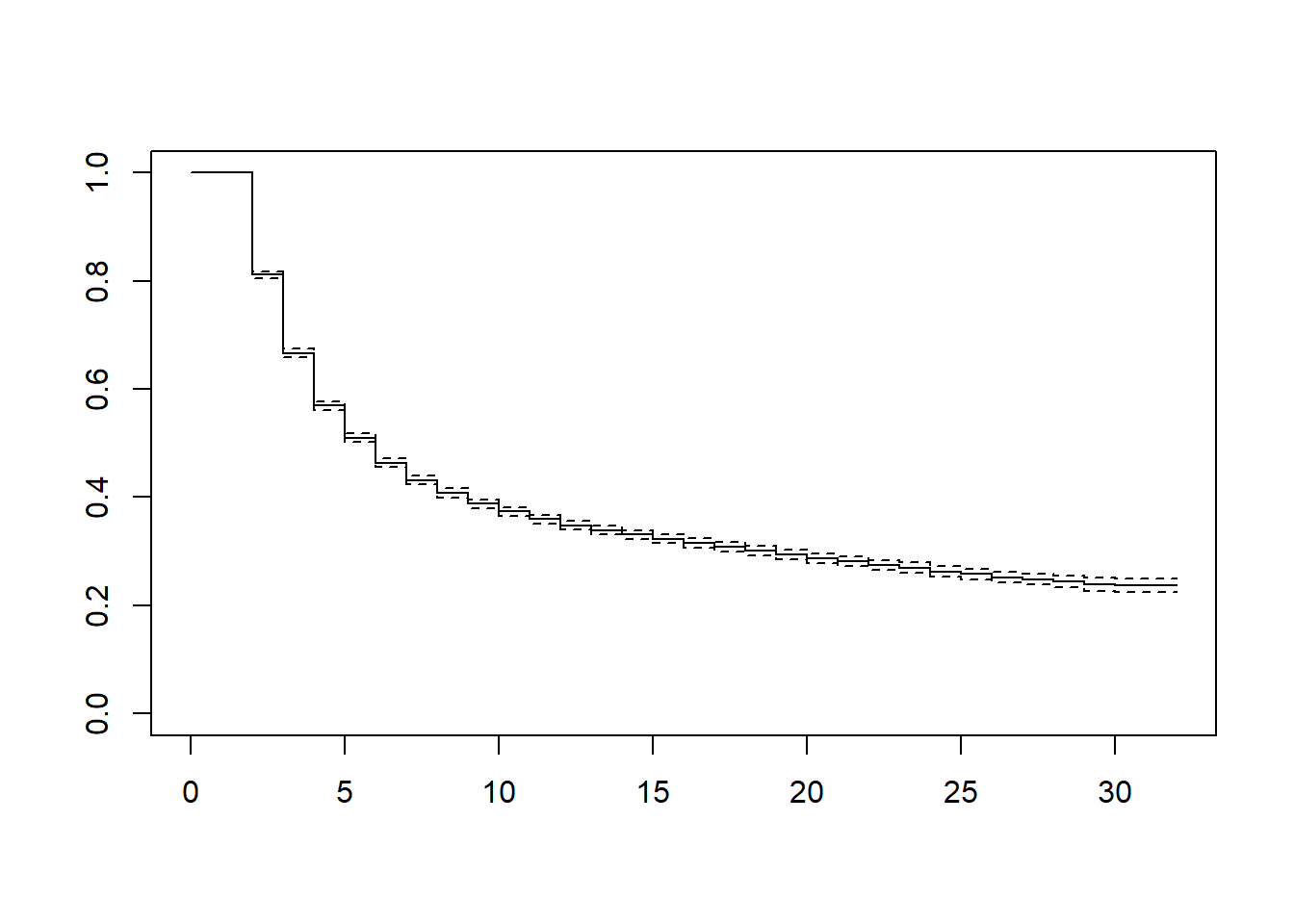

plot(KM2)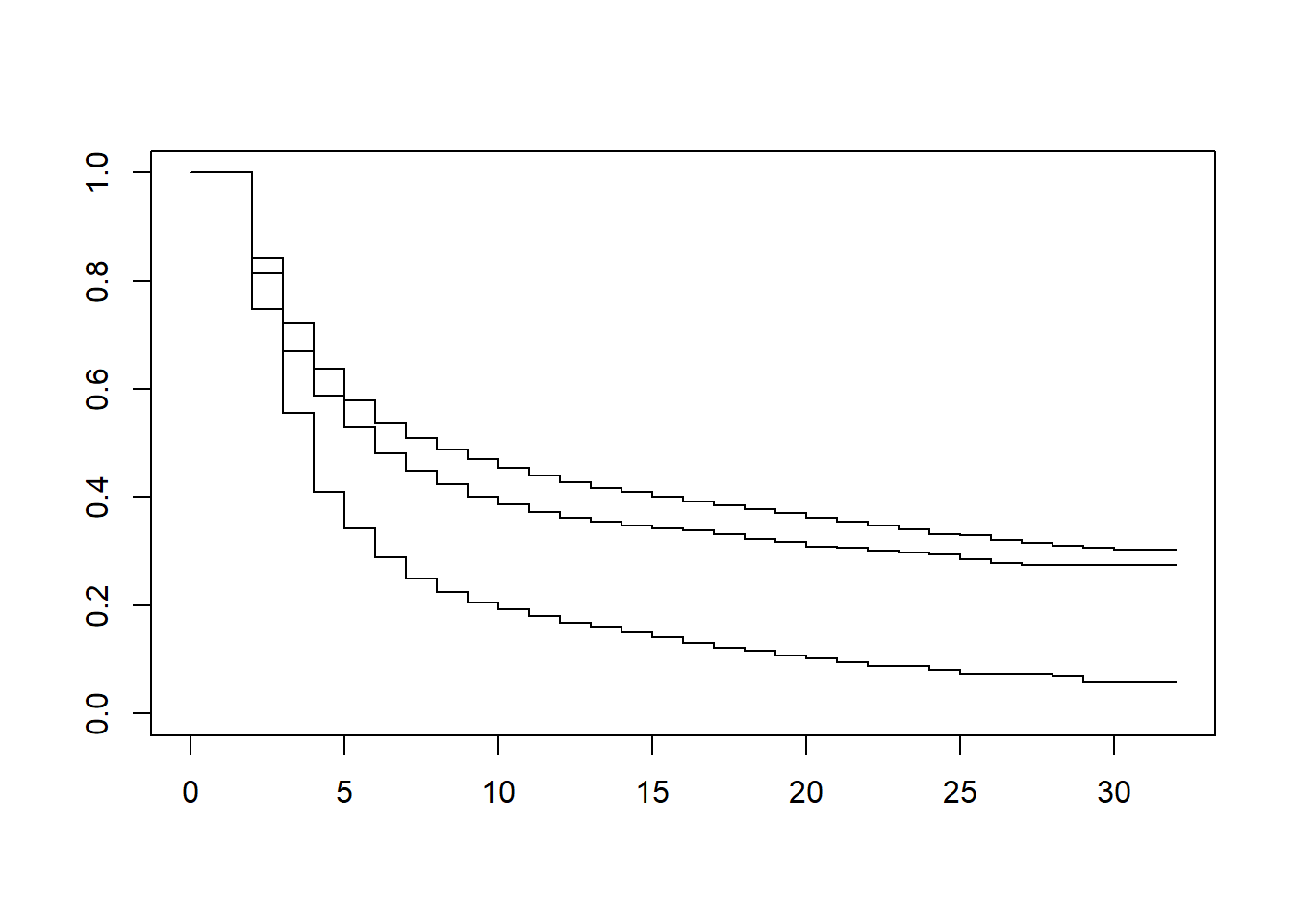

plot(KM3)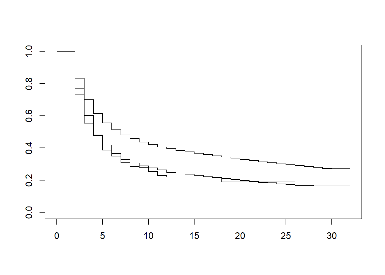

#MC1 <- flexsurvreg(Surv((time -1), time, inactive) ~ 1, data = df_ppf3, dist = "gengamma") # commented: no convergence
#MC2 <- flexsurvreg(Surv((time -1), time, inactive) ~ 1, data = df_ppf3, dist = "genf")     # commented: no convergence
MC3 <- flexsurvreg(Surv((time -1), time, inactive) ~ 1, data = df_ppf3, dist = "weibull")
MC4 <- flexsurvreg(Surv((time -1), time, inactive) ~ 1, data = df_ppf3, dist = "gamma")
MC5 <- flexsurvreg(Surv((time -1), time, inactive) ~ 1, data = df_ppf3, dist = "exp")
MC6 <- flexsurvreg(Surv((time -1), time, inactive) ~ 1, data = df_ppf3, dist = "llogis")
MC7 <- flexsurvreg(Surv((time -1), time, inactive) ~ 1, data = df_ppf3, dist = "gompertz")
MC8 <- flexsurvreg(Surv((time -1), time, inactive) ~ 1, data = df_ppf3, dist = "lognormal")

testdist <- AIC(MC3, MC4, MC5, MC6, MC7, MC8)
testdist[order(testdist$AIC),]

Model 1: Gender only

M1 <- flexsurvreg(Surv((time -1), time, inactive) ~ gender , data = df_ppf3, dist = "lognormal")

M1

## Call:
## flexsurvreg(formula = Surv((time - 1), time, inactive) ~ gender, 
##     data = df_ppf3, dist = "lognormal")
## 
## Estimates: 
##                data mean  est       L95%      U95%      se        exp(est)  L95%      U95%    
## meanlog              NA    2.19181   2.16380   2.21983   0.01429        NA        NA        NA
## sdlog                NA    1.06590   1.05003   1.08202   0.00816        NA        NA        NA
## genderwomen     0.32431   -0.19212  -0.23351  -0.15073   0.02112   0.82521   0.79175   0.86008
## gendermissing   0.15973   -0.62256  -0.66863  -0.57649   0.02351   0.53657   0.51241   0.56187
## 
## N = 118372,  Events: 9951,  Censored: 108421
## Total time at risk: 118372
## Log-likelihood = -32564.76, df = 4
## AIC = 65137.52

P-values

##       meanlog         sdlog   genderwomen gendermissing 
##             0             0             0             0

Model 2: Ethnicity only

M2 <- flexsurvreg(Surv((time -1), time, inactive) ~ ethnicity2 , data = df_ppf3, dist = "lognormal")

M2

## Call:
## flexsurvreg(formula = Surv((time - 1), time, inactive) ~ ethnicity2, 
##     data = df_ppf3, dist = "lognormal")
## 
## Estimates: 
##                     data mean  est       L95%      U95%      se        exp(est)  L95%      U95%    
## meanlog                   NA    2.11350   2.09063   2.13636   0.01167        NA        NA        NA
## sdlog                     NA    1.07443   1.05840   1.09070   0.00824        NA        NA        NA
## ethnicity2minority   0.01282   -0.45499  -0.58923  -0.32075   0.06849   0.63445   0.55475   0.72561
## ethnicity2other      0.24807   -0.37859  -0.41738  -0.33980   0.01979   0.68483   0.65877   0.71191
## 
## N = 118372,  Events: 9951,  Censored: 108421
## Total time at risk: 118372
## Log-likelihood = -32721.55, df = 4
## AIC = 65451.1

P-values

##            meanlog              sdlog ethnicity2minority    ethnicity2other 
##                  0                  0                  0                  0

Model 3: Gender and ethnicity, controls

M3 <- flexsurvreg(Surv((time -1), time, inactive) ~ gender + ethnicity2 + uni + field2 + phd_cohort + npubs_prev_s, data = df_ppf3, dist = "lognormal")

M3

## Call:
## flexsurvreg(formula = Surv((time - 1), time, inactive) ~ gender + 
##     ethnicity2 + uni + field2 + phd_cohort + npubs_prev_s, data = df_ppf3, 
##     dist = "lognormal")
## 
## Estimates: 
##                                           data mean  est        L95%       U95%       se       
## meanlog                                          NA   2.254134   2.172277   2.335991   0.041765
## sdlog                                            NA   0.847069   0.834590   0.859736   0.006415
## genderwomen                                0.324308  -0.084489  -0.118045  -0.050932   0.017121
## gendermissing                              0.159734  -0.436816  -0.475709  -0.397922   0.019844
## ethnicity2minority                         0.012824  -0.119125  -0.224714  -0.013536   0.053873
## ethnicity2other                            0.248065  -0.101543  -0.133789  -0.069298   0.016452
## uniLU                                      0.016947  -0.054197  -0.173059   0.064666   0.060645
## uniRU                                      0.211317  -0.205849  -0.284479  -0.127219   0.040118
## uniRUG                                     0.040846   0.608518   0.457734   0.759303   0.076932
## uniTUD                                     0.004131   0.367652   0.163204   0.572100   0.104312
## uniTUE                                     0.023840   0.503403   0.342315   0.664492   0.082190
## uniTI                                      0.010873  -0.435195  -0.578198  -0.292192   0.072962
## uniUM                                      0.096568  -0.023207  -0.109659   0.063245   0.044109
## uniUT                                      0.080543  -0.605701  -0.691606  -0.519796   0.043830
## uniUU                                      0.090376  -0.181588  -0.265715  -0.097462   0.042922
## uniUvA                                     0.121828  -0.049879  -0.136390   0.036633   0.044139
## uniVU                                      0.090748  -0.048208  -0.137242   0.040825   0.045426
## uniWUR                                     0.158940  -0.000619  -0.085835   0.084596   0.043478
## field2Physical and Mathematical Sciences   0.116016  -0.201981  -0.248623  -0.155340   0.023797
## field2Social and Behavioral Sciences       0.145904   0.193687   0.146858   0.240516   0.023893
## field2Engineering                          0.077620  -0.119362  -0.176828  -0.061897   0.029320
## field2Agricultural Sciences                0.085899   0.048752  -0.010329   0.107833   0.030144
## field2Humanities                           0.041429   0.293647   0.209210   0.378085   0.043081
## field2missing                              0.160798   0.290978   0.243449   0.338508   0.024250
## phd_cohort                                15.109840  -0.033922  -0.036236  -0.031609   0.001180
## npubs_prev_s                               0.479051   1.500639   1.434418   1.566861   0.033787
##                                           exp(est)   L95%       U95%     
## meanlog                                          NA         NA         NA
## sdlog                                            NA         NA         NA
## genderwomen                                0.918982   0.888656   0.950343
## gendermissing                              0.646090   0.621444   0.671714
## ethnicity2minority                         0.887697   0.798745   0.986556
## ethnicity2other                            0.903442   0.874775   0.933049
## uniLU                                      0.947246   0.841088   1.066802
## uniRU                                      0.813956   0.752406   0.880540
## uniRUG                                     1.837707   1.580489   2.136786
## uniTUD                                     1.444340   1.177277   1.771985
## uniTUE                                     1.654342   1.408203   1.943503
## uniTI                                      0.647138   0.560908   0.746625
## uniUM                                      0.977060   0.896139   1.065288
## uniUT                                      0.545692   0.500771   0.594642
## uniUU                                      0.833945   0.766658   0.907137
## uniUvA                                     0.951345   0.872502   1.037312
## uniVU                                      0.952935   0.871759   1.041670
## uniWUR                                     0.999381   0.917746   1.088278
## field2Physical and Mathematical Sciences   0.817110   0.779874   0.856124
## field2Social and Behavioral Sciences       1.213716   1.158189   1.271905
## field2Engineering                          0.887486   0.837924   0.939980
## field2Agricultural Sciences                1.049960   0.989724   1.113862
## field2Humanities                           1.341311   1.232703   1.459487
## field2missing                              1.337736   1.275641   1.402853
## phd_cohort                                 0.966647   0.964413   0.968886
## npubs_prev_s                               4.484555   4.197201   4.791582
## 
## N = 118372,  Events: 9951,  Censored: 108421
## Total time at risk: 118372
## Log-likelihood = -30292, df = 26
## AIC = 60636

P-values

##                                  meanlog                                    sdlog 
##                                   0.0000                                   0.0000 
##                              genderwomen                            gendermissing 
##                                   0.0000                                   0.0000 
##                       ethnicity2minority                          ethnicity2other 
##                                   0.0270                                   0.0000 
##                                    uniLU                                    uniRU 
##                                   0.3715                                   0.0000 
##                                   uniRUG                                   uniTUD 
##                                   0.0000                                   0.0004 
##                                   uniTUE                                    uniTI 
##                                   0.0000                                   0.0000 
##                                    uniUM                                    uniUT 
##                                   0.5988                                   0.0000 
##                                    uniUU                                   uniUvA 
##                                   0.0000                                   0.2585 
##                                    uniVU                                   uniWUR 
##                                   0.2886                                   0.9886 
## field2Physical and Mathematical Sciences     field2Social and Behavioral Sciences 
##                                   0.0000                                   0.0000 
##                        field2Engineering              field2Agricultural Sciences 
##                                   0.0000                                   0.1058 
##                         field2Humanities                            field2missing 
##                                   0.0000                                   0.0000 
##                               phd_cohort                             npubs_prev_s 
##                                   0.0000                                   0.0000

Average marginal effects (AMEs)

bootFunc <- function(data, i) {
  df <- data[i,] #bootstrap datasets
  
  
  M <- flexsurv::flexsurvreg(survival::Surv((time -1), time, inactive) ~ gender + ethnicity2 + uni + field2 + phd_cohort + npubs_prev_s, data = df, dist = "lognormal")
  
  suppressWarnings({
  
    dfmaj <- dfmin <- dfmen <- dfwomen <- df
    dfwomen$gender <- "women" # one dataset of all women
    dfmen$gender <- "men" # one dataset of all men
    dfmin$ethnicity2 <- "minority" # one dataset all minority
    dfmaj$ethnicity2 <- "majority" # one dataset all majority
    
    dfwomen$gender <- factor(dfwomen$gender, levels=levels(df$gender))
    dfmen$gender <- factor(dfmen$gender, levels=levels(df$gender))
    dfmin$ethnicity2 <- factor(dfmin$ethnicity2, levels=levels(df$ethnicity2))
    dfmaj$ethnicity2 <- factor(dfmaj$ethnicity2, levels=levels(df$ethnicity2))

    #calculate the predicted probabilities for gender
    pw <- as.numeric(unlist(predict(M, type="response", newdata=dfwomen)))
    pm <- as.numeric(unlist(predict(M, type="response", newdata=dfmen)))
    
    # average marginal effects
    AME_gender <- mean(pw - pm)
    
    #calculate the predicted probabilities for ethnicity
    pmn <- as.numeric(unlist(predict(M, type="response", newdata=dfmin)))
    pmj <- as.numeric(unlist(predict(M, type="response", newdata=dfmaj)))

    # average marginal effects
    AME_ethnicity <- mean(pmn - pmj)
    
  })
  
  c(AME_gender, AME_ethnicity)
   #save results
}

b3 <- boot(df_ppf3, bootFunc, R = 999, parallel="snow", ncpus=10)


fsave(b3, file = "boot3.rda", location = "./results/stopping/")

original <- b3$t0
bias <- colMeans(b3$t) - b3$t0
se <- apply(b3$t, 2, sd)

boot.df3 <- data.frame(original=original, bias=bias, se=se)
row.names(boot.df3) <- c("AME_gender", "AME_ethnicity")

boot.df3$t <- (boot.df3$original / boot.df3$se)

round(boot.df3, 5)

##               original     bias      se        t
## AME_gender    -1.65428 -0.00432 0.31677 -5.22231
## AME_ethnicity -2.18740  0.04751 0.84055 -2.60236

Model 4: Gender + ethnicity + cohort x gender + cohort x ethnicity + controls

M4 <- flexsurvreg(Surv((time -1), time, inactive) ~ gender + ethnicity2 + uni + field2 + phd_cohort + npubs_prev_s + phd_cohort*gender + phd_cohort*ethnicity2, data = df_ppf3, dist = "lognormal")

M4

## Call:
## flexsurvreg(formula = Surv((time - 1), time, inactive) ~ gender + 
##     ethnicity2 + uni + field2 + phd_cohort + npubs_prev_s + phd_cohort * 
##     gender + phd_cohort * ethnicity2, data = df_ppf3, dist = "lognormal")
## 
## Estimates: 
##                                           data mean  est        L95%       U95%       se       
## meanlog                                          NA   2.241756   2.152108   2.331405   0.045740
## sdlog                                            NA   0.845462   0.833004   0.858107   0.006404
## genderwomen                                0.324308   0.021328  -0.074926   0.117582   0.049110
## gendermissing                              0.159734  -0.656435  -0.759920  -0.552949   0.052800
## ethnicity2minority                         0.012824  -0.138562  -0.533041   0.255916   0.201268
## ethnicity2other                            0.248065  -0.020699  -0.118039   0.076640   0.049664
## uniLU                                      0.016947  -0.036353  -0.155113   0.082408   0.060593
## uniRU                                      0.211317  -0.195520  -0.274085  -0.116955   0.040085
## uniRUG                                     0.040846   0.606243   0.455623   0.756863   0.076848
## uniTUD                                     0.004131   0.392737   0.188261   0.597213   0.104326
## uniTUE                                     0.023840   0.515919   0.354808   0.677030   0.082201
## uniTI                                      0.010873  -0.416125  -0.559084  -0.273166   0.072940
## uniUM                                      0.096568  -0.004576  -0.091134   0.081982   0.044163
## uniUT                                      0.080543  -0.584547  -0.670719  -0.498374   0.043966
## uniUU                                      0.090376  -0.164626  -0.248936  -0.080315   0.043016
## uniUvA                                     0.121828  -0.034374  -0.121055   0.052307   0.044226
## uniVU                                      0.090748  -0.033359  -0.122402   0.055684   0.045431
## uniWUR                                     0.158940   0.010904  -0.074224   0.096032   0.043434
## field2Physical and Mathematical Sciences   0.116016  -0.202237  -0.248801  -0.155672   0.023758
## field2Social and Behavioral Sciences       0.145904   0.190841   0.144093   0.237589   0.023852
## field2Engineering                          0.077620  -0.118354  -0.175720  -0.060987   0.029269
## field2Agricultural Sciences                0.085899   0.044306  -0.014673   0.103284   0.030092
## field2Humanities                           0.041429   0.293140   0.208847   0.377434   0.043008
## field2missing                              0.160798   0.291224   0.243740   0.338708   0.024227
## phd_cohort                                15.109840  -0.033855  -0.037081  -0.030628   0.001646
## npubs_prev_s                               0.479051   1.496518   1.430389   1.562648   0.033740
## genderwomen:phd_cohort                     5.472333  -0.005237  -0.010027  -0.000446   0.002444
## gendermissing:phd_cohort                   2.550983   0.012432   0.006944   0.017920   0.002800
## ethnicity2minority:phd_cohort              0.242718   0.000462  -0.017883   0.018808   0.009360
## ethnicity2other:phd_cohort                 4.313131  -0.004433  -0.009240   0.000374   0.002453
##                                           exp(est)   L95%       U95%     
## meanlog                                          NA         NA         NA
## sdlog                                            NA         NA         NA
## genderwomen                                1.021557   0.927813   1.124774
## gendermissing                              0.518697   0.467704   0.575251
## ethnicity2minority                         0.870609   0.586818   1.291645
## ethnicity2other                            0.979513   0.888661   1.079654
## uniLU                                      0.964300   0.856318   1.085899
## uniRU                                      0.822407   0.760267   0.889625
## uniRUG                                     1.833530   1.577155   2.131579
## uniTUD                                     1.481029   1.207148   1.817048
## uniTUE                                     1.675177   1.425907   1.968024
## uniTI                                      0.659598   0.571733   0.760966
## uniUM                                      0.995435   0.912896   1.085436
## uniUT                                      0.557359   0.511341   0.607517
## uniUU                                      0.848211   0.779630   0.922825
## uniUvA                                     0.966210   0.885985   1.053699
## uniVU                                      0.967191   0.884793   1.057263
## uniWUR                                     1.010964   0.928463   1.100795
## field2Physical and Mathematical Sciences   0.816902   0.779735   0.855840
## field2Social and Behavioral Sciences       1.210267   1.154992   1.268188
## field2Engineering                          0.888382   0.838853   0.940835
## field2Agricultural Sciences                1.045302   0.985434   1.108807
## field2Humanities                           1.340631   1.232256   1.458537
## field2missing                              1.338065   1.276013   1.403134
## phd_cohort                                 0.966712   0.963598   0.969836
## npubs_prev_s                               4.466113   4.180324   4.771440
## genderwomen:phd_cohort                     0.994777   0.990023   0.999554
## gendermissing:phd_cohort                   1.012510   1.006968   1.018082
## ethnicity2minority:phd_cohort              1.000462   0.982276   1.018986
## ethnicity2other:phd_cohort                 0.995577   0.990802   1.000374
## 
## N = 118372,  Events: 9951,  Censored: 108421
## Total time at risk: 118372
## Log-likelihood = -30274.33, df = 30
## AIC = 60608.66

P-values

##                                  meanlog                                    sdlog 
##                                   0.0000                                   0.0000 
##                              genderwomen                            gendermissing 
##                                   0.6641                                   0.0000 
##                       ethnicity2minority                          ethnicity2other 
##                                   0.4912                                   0.6768 
##                                    uniLU                                    uniRU 
##                                   0.5485                                   0.0000 
##                                   uniRUG                                   uniTUD 
##                                   0.0000                                   0.0002 
##                                   uniTUE                                    uniTI 
##                                   0.0000                                   0.0000 
##                                    uniUM                                    uniUT 
##                                   0.9175                                   0.0000 
##                                    uniUU                                   uniUvA 
##                                   0.0001                                   0.4370 
##                                    uniVU                                   uniWUR 
##                                   0.4628                                   0.8018 
## field2Physical and Mathematical Sciences     field2Social and Behavioral Sciences 
##                                   0.0000                                   0.0000 
##                        field2Engineering              field2Agricultural Sciences 
##                                   0.0001                                   0.1409 
##                         field2Humanities                            field2missing 
##                                   0.0000                                   0.0000 
##                               phd_cohort                             npubs_prev_s 
##                                   0.0000                                   0.0000 
##                   genderwomen:phd_cohort                 gendermissing:phd_cohort 
##                                   0.0322                                   0.0000 
##            ethnicity2minority:phd_cohort               ethnicity2other:phd_cohort 
##                                   0.9606                                   0.0707

Average marginal effects (AMEs)

bootFunc <- function(data, i) {
  df <- data[i,] #bootstrap datasets
  
  
  M <- flexsurv::flexsurvreg(survival::Surv((time -1), time, inactive) ~ gender + ethnicity2 + uni + field2 + phd_cohort + npubs_prev_s + phd_cohort*gender + phd_cohort*ethnicity2, data = df, dist = "lognormal")
  
  suppressWarnings({
  
    dfmaj <- dfmin <- dfmen <- dfwomen <- df
    dfwomen$gender <- "women" # one dataset of all women
    dfmen$gender <- "men" # one dataset of all men
    dfmin$ethnicity2 <- "minority" # one dataset all minority
    dfmaj$ethnicity2 <- "majority" # one dataset all majority
    
    dfwomen$gender <- factor(dfwomen$gender, levels=levels(df$gender))
    dfmen$gender <- factor(dfmen$gender, levels=levels(df$gender))
    dfmin$ethnicity2 <- factor(dfmin$ethnicity2, levels=levels(df$ethnicity2))
    dfmaj$ethnicity2 <- factor(dfmaj$ethnicity2, levels=levels(df$ethnicity2))

    #calculate the predicted probabilities for gender
    pw <- as.numeric(unlist(predict(M, type="response", newdata=dfwomen)))
    pm <- as.numeric(unlist(predict(M, type="response", newdata=dfmen)))
    
    # average marginal effects
    AME_gender <- mean(pw - pm)
    
    #calculate the predicted probabilities for ethnicity
    pmn <- as.numeric(unlist(predict(M, type="response", newdata=dfmin)))
    pmj <- as.numeric(unlist(predict(M, type="response", newdata=dfmaj)))

    # average marginal effects
    AME_ethnicity <- mean(pmn - pmj)
    
    
    # cohort interactions
    
    s <- 0.1
    # copying our data into separate dataframes
    dfwomencp <- dfwomencm <- dfmencp <- dfmencm <- df
    dfmincp <- dfmincm <- dfmajcp <- dfmajcm <- df
    
    # assigning gender to each of the dataframes
    dfwomencp$gender <- dfwomencm$gender <- "women"
    dfmencp$gender <- dfmencm$gender <- "men"
    dfwomencp$gender <- factor(dfwomencp$gender, levels=levels(df$gender))
    dfwomencm$gender <- factor(dfwomencm$gender, levels=levels(df$gender))
    dfmencp$gender <- factor(dfmencp$gender, levels=levels(df$gender))
    dfmencm$gender <- factor(dfmencm$gender, levels=levels(df$gender))
    
    # assigning ethnicity to the dataframes
    dfmincp$ethnicity2 <- dfmincm$ethnicity2 <- "minority"
    dfmajcp$ethnicity2 <- dfmajcm$ethnicity2 <- "majority"
    dfmincp$ethnicity2 <- factor(dfmincp$ethnicity2, levels=levels(df$ethnicity2))
    dfmincm$ethnicity2 <- factor(dfmincm$ethnicity2, levels=levels(df$ethnicity2))
    dfmajcp$ethnicity2 <- factor(dfmajcp$ethnicity2, levels=levels(df$ethnicity2))
    dfmajcm$ethnicity2 <- factor(dfmajcm$ethnicity2, levels=levels(df$ethnicity2))
    
    
    # adding/subtracting small changes PhD cohort
    dfwomencp$phd_cohort <- dfmencp$phd_cohort <- df$phd_cohort + s
    dfwomencm$phd_cohort <- dfmencm$phd_cohort <- df$phd_cohort - s
    
    dfmajcp$phd_cohort <- dfmincp$phd_cohort <- df$phd_cohort + s
    dfmajcm$phd_cohort <- dfmincm$phd_cohort <- df$phd_cohort - s
    
    # calculating predicted probabilities
    pwp <- as.numeric(unlist(predict(M, type="response", newdata=dfwomencp)))
    pwm <- as.numeric(unlist(predict(M, type="response", newdata=dfwomencm)))
    pmp <- as.numeric(unlist(predict(M, type="response", newdata=dfmencp)))
    pmm <- as.numeric(unlist(predict(M, type="response", newdata=dfmencm)))
    
    pnp <- as.numeric(unlist(predict(M, type="response", newdata=dfmincp)))
    pnm <- as.numeric(unlist(predict(M, type="response", newdata=dfmincm)))
    pjp <- as.numeric(unlist(predict(M, type="response", newdata=dfmajcp)))
    pjm <- as.numeric(unlist(predict(M, type="response", newdata=dfmajcm)))
    
    
# marginal effects
AME_gendercoh <- mean(((pwp - pmp) - (pwm - pmm)) / (2*s))

AME_ethnicitycoh <- mean(((pnp - pjp) - (pnm - pjm)) / (2*s))

  })
  
  c(AME_gender, AME_ethnicity, AME_gendercoh, AME_ethnicitycoh)
   #save results
}

b4 <- boot(df_ppf3, bootFunc, R = 999, parallel="snow", ncpus=10)


fsave(b4, file = "boot4.rda", location = "./results/stopping/")

original <- b4$t0
bias <- colMeans(b4$t) - b4$t0
se <- apply(b4$t, 2, sd)

boot.df4 <- data.frame(original=original, bias=bias, se=se)
row.names(boot.df4) <- c("AME_gender", "AME_ethnicity", "AME_gender-coh", "AME_ethnicity-coh")

boot.df4$t <- (boot.df4$original / boot.df4$se)

round(boot.df4, 5)

##                   original     bias      se        t
## AME_gender        -0.78358  0.00137 0.51239 -1.52926
## AME_ethnicity     -2.43144  0.15562 1.67483 -1.45175
## AME_gender-coh    -0.07530 -0.00054 0.06601 -1.14074
## AME_ethnicity-coh  0.09160 -0.01590 0.20778  0.44085

Table 4

columns <- c(rep(c("B", "C.I."), 4))
rows <- c("<strong>Shape</strong></p>", "<strong>Scale</strong></p>", "Gender: ref=men" ,"Women", "Missing gender", "Ethnicity: ref=majority","Minority", "Other", "University: ref=Erasmus University", "Leiden University", "Radboud University", "University of Groningen", "Delft University of Technology", "Eindhoven University of Technology", "Tilburg University", "Maastricht University", "University of Twente", "Utrecht University", "University of Amsterdam", "Vrije Universiteit Amsterdam", "Wageningen University and Research Centre", "Field: ref=Biological and Health Sciences", "Physical and mathematical sciences", "Social and behavioral sciences", "Engineering", "Agricultural sciences", "Humanities", "Missing field", "<strong>PhD cohort</strong></p>", "<strong>Previous publications</strong></p>", "Cohort interactions","PhD cohort * women", "PhD cohort * missing gender", "PhD cohort * ethnic minority", "PhD cohort * other ethnicity", "<strong>AIC", "<strong>N")


t4 <- data.frame(matrix(nrow=length(rows), ncol=length(columns)))
colnames(t4) <- columns
rownames(t4) <- rows



# Model 1
t4[c(1,2,4,5),1] <- format(round(as.numeric(M1$coef), 2), nsmall=2) # estimates
t4[c(1,2),2] <- paste0("[", format(round(log(M1$res[c(1,2),2]), 2), nsmall=2), " , ", format(round(log(M1$res[c(1,2),3]), 2), nsmall=2), "]") # CI for shape and scale
t4[c(4,5),2] <- paste0("[", format(round(M1$res[c(3,4),2], 2), nsmall=2), " , ", format(round(M1$res[c(3,4),3], 3), nsmall=2), "]") # CI for other covariates


# Model 2
t4[c(1,2,7,8),3] <- format(round(M2$coef, 2), nsmall=2)
t4[c(1,2),4] <- paste0("[", format(round(log(M2$res[c(1,2),2]), 2), nsmall=2), " , ", format(round(log(M2$res[c(1,2),3]), 2), nsmall=2), "]")
t4[c(7,8),4] <- paste0("[", format(round(M2$res[c(3,4),2], 2), nsmall=2), " , ", format(round(M2$res[c(3,4),3], 2), nsmall=2), "]")

# Model 3
t4[c(1,2,4,5,7,8,10:21,23:30),5] <- format(round(M3$coef, 2), nsmall=2)
#t4[c(1,2), 6] <- paste("[", round(log(M3$res[c(1,2),2]), 3), ",", round(log(M3$res[c(1,2),3]), 3), "]")
t4[c(1,2,4,5,7,8,10:21,23:30), 6] <- paste0("[", format(round(M3$res[c(1,2,3:26),2], 2), nsmall=2), " , ", format(round(M3$res[c(1,2,3:26),3], 2), nsmall=2), "]")

# Model 4 
t4[c(1,2,4,5,7,8,10:21,23:30,32:35),7] <- format(round(M4$coef, 2), nsmall=2)
#t4[c(1,2), 8] <- paste("[", round(log(M4$res[c(1:2),2]), 3), ",", round(log(M4$res[c(1:2),3]), 3), "]")
t4[c(1,2,4,5,7,8,10:21,23:30,32:35), 8] <- paste0("[", format(round(M4$res[c(1,2,3:30),2], 2), nsmall=2), " , ", format(round(M4$res[c(1,2,3:30),3], 2), nsmall=2), "]")


# AIC
t4[36,1] <- round(M1$AIC, 0)
t4[36,3] <- round(M2$AIC, 0)
t4[36,5] <- round(M3$AIC, 0)
t4[36,7] <- round(M4$AIC, 0)

# sample size
t4[37, c(1,3,5,7)] <- rep(nrow(df_ppf3[!duplicated(df_ppf3$id),]), 4)


t4[is.na(t4)] <- ""

t4 %>%
  kable(format = 'html', caption = '<b>Table 4.</b> Log-normal regression analyses on stopping to publish', escape=FALSE) %>%
  add_header_above(.,c(' '=1, 'Model 1'=2, 'Model 2'=2, 'Model 3'=2, 'Model 4'=2), escape = FALSE, bold = TRUE) %>%
  row_spec(row=c(3,6,9,22,31), bold=T) %>%
  kable_classic(full_width = F, html_font = "Cambria") %>%
  kable_styling(font_size = 11) -> table4

table4

**Table 4.** Log-normal regression analyses on stopping to publish
	Model 1		Model 2		Model 3		Model 4
	B	C.I.	B	C.I.	B	C.I.	B	C.I.
Shape	2.19	[0.77 , 0.80]	2.11	[0.74 , 0.76]	2.25	[ 2.17 , 2.34]	2.24	[ 2.15 , 2.33]
Scale	0.06	[0.05 , 0.08]	0.07	[0.06 , 0.09]	-0.17	[ 0.83 , 0.86]	-0.17	[ 0.83 , 0.86]
Gender: ref=men
Women	-0.19	[-0.23 , -0.151]			-0.08	[-0.12 , -0.05]	0.02	[-0.07 , 0.12]
Missing gender	-0.62	[-0.67 , -0.576]			-0.44	[-0.48 , -0.40]	-0.66	[-0.76 , -0.55]
Ethnicity: ref=majority
Minority			-0.45	[-0.59 , -0.32]	-0.12	[-0.22 , -0.01]	-0.14	[-0.53 , 0.26]
Other			-0.38	[-0.42 , -0.34]	-0.10	[-0.13 , -0.07]	-0.02	[-0.12 , 0.08]
University: ref=Erasmus University
Leiden University					-0.05	[-0.17 , 0.06]	-0.04	[-0.16 , 0.08]
Radboud University					-0.21	[-0.28 , -0.13]	-0.20	[-0.27 , -0.12]
University of Groningen					0.61	[ 0.46 , 0.76]	0.61	[ 0.46 , 0.76]
Delft University of Technology					0.37	[ 0.16 , 0.57]	0.39	[ 0.19 , 0.60]
Eindhoven University of Technology					0.50	[ 0.34 , 0.66]	0.52	[ 0.35 , 0.68]
Tilburg University					-0.44	[-0.58 , -0.29]	-0.42	[-0.56 , -0.27]
Maastricht University					-0.02	[-0.11 , 0.06]	0.00	[-0.09 , 0.08]
University of Twente					-0.61	[-0.69 , -0.52]	-0.58	[-0.67 , -0.50]
Utrecht University					-0.18	[-0.27 , -0.10]	-0.16	[-0.25 , -0.08]
University of Amsterdam					-0.05	[-0.14 , 0.04]	-0.03	[-0.12 , 0.05]
Vrije Universiteit Amsterdam					-0.05	[-0.14 , 0.04]	-0.03	[-0.12 , 0.06]
Wageningen University and Research Centre					0.00	[-0.09 , 0.08]	0.01	[-0.07 , 0.10]
Field: ref=Biological and Health Sciences
Physical and mathematical sciences					-0.20	[-0.25 , -0.16]	-0.20	[-0.25 , -0.16]
Social and behavioral sciences					0.19	[ 0.15 , 0.24]	0.19	[ 0.14 , 0.24]
Engineering					-0.12	[-0.18 , -0.06]	-0.12	[-0.18 , -0.06]
Agricultural sciences					0.05	[-0.01 , 0.11]	0.04	[-0.01 , 0.10]
Humanities					0.29	[ 0.21 , 0.38]	0.29	[ 0.21 , 0.38]
Missing field					0.29	[ 0.24 , 0.34]	0.29	[ 0.24 , 0.34]
PhD cohort					-0.03	[-0.04 , -0.03]	-0.03	[-0.04 , -0.03]
Previous publications					1.50	[ 1.43 , 1.57]	1.50	[ 1.43 , 1.56]
Cohort interactions
PhD cohort * women							-0.01	[-0.01 , 0.00]
PhD cohort * missing gender							0.01	[ 0.01 , 0.02]
PhD cohort * ethnic minority							0.00	[-0.02 , 0.02]
PhD cohort * other ethnicity							0.00	[-0.01 , 0.00]
AIC	65138		65451		60636		60609
N	15021		15021		15021		15021

Robustness checks

R1: 5-year publication window

R1 <- flexsurvreg(Surv((time -1), time, inactive) ~ gender , data = df_ppf5, dist = "lognormal")
R1

R2 <- flexsurvreg(Surv((time -1), time, inactive) ~ ethnicity2 , data = df_ppf5, dist = "lognormal")
R2

R3 <- flexsurvreg(Surv((time -1), time, inactive) ~ gender + ethnicity2 + uni + field2 + phd_cohort + npubs_prev_s, data = df_ppf5, dist = "lognormal")
R3

R4 <- flexsurvreg(Surv((time -1), time, inactive) ~ gender + ethnicity2 + uni + field2 + phd_cohort + npubs_prev_s + phd_cohort*gender + phd_cohort*ethnicity2, data = df_ppf5, dist = "lognormal")
R4

AMEs Model 3 (no SEs)

dfmaj <- dfmin <- dfmen <- dfwomen <- df_ppf5
    dfwomen$gender <- "women" # one dataset of all women
    dfmen$gender <- "men" # one dataset of all men
    dfmin$ethnicity2 <- "minority" # one dataset all minority
    dfmaj$ethnicity2 <- "majority" # one dataset all majority
    
    dfwomen$gender <- factor(dfwomen$gender, levels=levels(df_ppf5$gender))
    dfmen$gender <- factor(dfmen$gender, levels=levels(df_ppf5$gender))
    dfmin$ethnicity2 <- factor(dfmin$ethnicity2, levels=levels(df_ppf5$ethnicity2))
    dfmaj$ethnicity2 <- factor(dfmaj$ethnicity2, levels=levels(df_ppf5$ethnicity2))

    #calculate the predicted probabilities for gender
    pw <- as.numeric(unlist(predict(R3, type="response", newdata=dfwomen)))
    pm <- as.numeric(unlist(predict(R3, type="response", newdata=dfmen)))
    
    # average marginal effects
    AME_gender <- mean(pw - pm)
    
    #calculate the predicted probabilities for ethnicity
    pmn <- as.numeric(unlist(predict(R3, type="response", newdata=dfmin)))
    pmj <- as.numeric(unlist(predict(R3, type="response", newdata=dfmaj)))

    # average marginal effects
    AME_ethnicity <- mean(pmn - pmj)
    
    
AME_gender
AME_ethnicity

AMEs Model 4 (no SEs)

    dfmaj <- dfmin <- dfmen <- dfwomen <- df_ppf5
    dfwomen$gender <- "women" # one dataset of all women
    dfmen$gender <- "men" # one dataset of all men
    dfmin$ethnicity2 <- "minority" # one dataset all minority
    dfmaj$ethnicity2 <- "majority" # one dataset all majority
    
    dfwomen$gender <- factor(dfwomen$gender, levels=levels(df_ppf5$gender))
    dfmen$gender <- factor(dfmen$gender, levels=levels(df_ppf5$gender))
    dfmin$ethnicity2 <- factor(dfmin$ethnicity2, levels=levels(df_ppf5$ethnicity2))
    dfmaj$ethnicity2 <- factor(dfmaj$ethnicity2, levels=levels(df_ppf5$ethnicity2))

    #calculate the predicted probabilities for gender
    pw <- as.numeric(unlist(predict(R4, type="response", newdata=dfwomen)))
    pm <- as.numeric(unlist(predict(R4, type="response", newdata=dfmen)))
    
    # average marginal effects
    AME_gender <- mean(pw - pm)
    
    #calculate the predicted probabilities for ethnicity
    pmn <- as.numeric(unlist(predict(R4, type="response", newdata=dfmin)))
    pmj <- as.numeric(unlist(predict(R4, type="response", newdata=dfmaj)))

    # average marginal effects
    AME_ethnicity <- mean(pmn - pmj)
    
    
    # cohort interactions
    
    s <- 0.1
    # copying our data into separate dataframes
    dfwomencp <- dfwomencm <- dfmencp <- dfmencm <- df_ppf5
    dfmincp <- dfmincm <- dfmajcp <- dfmajcm <- df_ppf5
    
    # assigning gender to each of the dataframes
    dfwomencp$gender <- dfwomencm$gender <- "women"
    dfmencp$gender <- dfmencm$gender <- "men"
    dfwomencp$gender <- factor(dfwomencp$gender, levels=levels(df_ppf5$gender))
    dfwomencm$gender <- factor(dfwomencm$gender, levels=levels(df_ppf5$gender))
    dfmencp$gender <- factor(dfmencp$gender, levels=levels(df_ppf5$gender))
    dfmencm$gender <- factor(dfmencm$gender, levels=levels(df_ppf5$gender))
    
    # assigning ethnicity to the dataframes
    dfmincp$ethnicity2 <- dfmincm$ethnicity2 <- "minority"
    dfmajcp$ethnicity2 <- dfmajcm$ethnicity2 <- "majority"
    dfmincp$ethnicity2 <- factor(dfmincp$ethnicity2, levels=levels(df_ppf5$ethnicity2))
    dfmincm$ethnicity2 <- factor(dfmincm$ethnicity2, levels=levels(df_ppf5$ethnicity2))
    dfmajcp$ethnicity2 <- factor(dfmajcp$ethnicity2, levels=levels(df_ppf5$ethnicity2))
    dfmajcm$ethnicity2 <- factor(dfmajcm$ethnicity2, levels=levels(df_ppf5$ethnicity2))
    
    
    # adding/subtracting small changes PhD cohort
    dfwomencp$phd_cohort <- dfmencp$phd_cohort <- df_ppf5$phd_cohort + s
    dfwomencm$phd_cohort <- dfmencm$phd_cohort <- df_ppf5$phd_cohort - s
    
    dfmajcp$phd_cohort <- dfmincp$phd_cohort <- df_ppf5$phd_cohort + s
    dfmajcm$phd_cohort <- dfmincm$phd_cohort <- df_ppf5$phd_cohort - s
    
    # calculating predicted probabilities
    pwp <- as.numeric(unlist(predict(R4, type="response", newdata=dfwomencp)))
    pwm <- as.numeric(unlist(predict(R4, type="response", newdata=dfwomencm)))
    pmp <- as.numeric(unlist(predict(R4, type="response", newdata=dfmencp)))
    pmm <- as.numeric(unlist(predict(R4, type="response", newdata=dfmencm)))
    
    pnp <- as.numeric(unlist(predict(R4, type="response", newdata=dfmincp)))
    pnm <- as.numeric(unlist(predict(R4, type="response", newdata=dfmincm)))
    pjp <- as.numeric(unlist(predict(R4, type="response", newdata=dfmajcp)))
    pjm <- as.numeric(unlist(predict(R4, type="response", newdata=dfmajcm)))
    
    
# marginal effects
AME_gendercoh <- mean(((pwp - pmp) - (pwm - pmm)) / (2*s))

AME_ethnicitycoh <- mean(((pnp - pjp) - (pnm - pjm)) / (2*s))

Model 3 SEs

bootFunc <- function(data, i) {
  df <- data[i,] #bootstrap datasets
  
  
  M <- flexsurv::flexsurvreg(survival::Surv((time -1), time, inactive) ~ gender + ethnicity2 + uni + field2 + phd_cohort + npubs_prev_s, data = df, dist = "lognormal")
  
  suppressWarnings({
  
    dfmaj <- dfmin <- dfmen <- dfwomen <- df
    dfwomen$gender <- "women" # one dataset of all women
    dfmen$gender <- "men" # one dataset of all men
    dfmin$ethnicity2 <- "minority" # one dataset all minority
    dfmaj$ethnicity2 <- "majority" # one dataset all majority
    
    dfwomen$gender <- factor(dfwomen$gender, levels=levels(df$gender))
    dfmen$gender <- factor(dfmen$gender, levels=levels(df$gender))
    dfmin$ethnicity2 <- factor(dfmin$ethnicity2, levels=levels(df$ethnicity2))
    dfmaj$ethnicity2 <- factor(dfmaj$ethnicity2, levels=levels(df$ethnicity2))

    #calculate the predicted probabilities for gender
    pw <- as.numeric(unlist(predict(M, type="response", newdata=dfwomen)))
    pm <- as.numeric(unlist(predict(M, type="response", newdata=dfmen)))
    
    # average marginal effects
    AME_gender <- mean(pw - pm)
    
    #calculate the predicted probabilities for ethnicity
    pmn <- as.numeric(unlist(predict(M, type="response", newdata=dfmin)))
    pmj <- as.numeric(unlist(predict(M, type="response", newdata=dfmaj)))

    # average marginal effects
    AME_ethnicity <- mean(pmn - pmj)
    
  })
  
  c(AME_gender, AME_ethnicity)
   #save results
}

b3 <- boot(df_ppf5, bootFunc, R = 100, parallel="snow", ncpus=10)


fsave(b3, file = "boot3_R1.rda", location = "./results/stopping/robustness/")

original <- b3$t0
bias <- colMeans(b3$t) - b3$t0
se <- apply(b3$t, 2, sd)

boot.df3 <- data.frame(original=original, bias=bias, se=se)
row.names(boot.df3) <- c("AME_gender", "AME_ethnicity")

boot.df3$t <- (boot.df3$original / boot.df3$se)

round(boot.df3, 5)

##               original     bias se  t
## AME_gender    -4.23738 -1.02307 NA NA
## AME_ethnicity -6.24852 -2.96893 NA NA

R2: ethnicity-missing included separately

R5 <- flexsurvreg(Surv((time -1), time, inactive) ~ ethnicity3 , data = df_ppf3, dist = "lognormal")
R5

R6 <- flexsurvreg(Surv((time -1), time, inactive) ~ gender + ethnicity3 + uni + field2 + phd_cohort + npubs_prev_s, data = df_ppf3, dist = "lognormal")
R6

R7 <- flexsurvreg(Surv((time -1), time, inactive) ~ gender + ethnicity3 + uni + field2 + phd_cohort + npubs_prev_s + phd_cohort*gender + phd_cohort*ethnicity2, data = df_ppf3, dist = "lognormal")
R7

AMEs Model 3 (no SEs)

dfmaj <- dfmin <- dfmen <- dfwomen <- df_ppf5
    dfwomen$gender <- "women" # one dataset of all women
    dfmen$gender <- "men" # one dataset of all men
    dfmin$ethnicity3 <- "minority" # one dataset all minority
    dfmaj$ethnicity3 <- "majority" # one dataset all majority
    
    dfwomen$gender <- factor(dfwomen$gender, levels=levels(df_ppf5$gender))
    dfmen$gender <- factor(dfmen$gender, levels=levels(df_ppf5$gender))
    dfmin$ethnicity3 <- factor(dfmin$ethnicity3, levels=levels(df_ppf5$ethnicity3))
    dfmaj$ethnicity3 <- factor(dfmaj$ethnicity3, levels=levels(df_ppf5$ethnicity3))

    #calculate the predicted probabilities for gender
    pw <- as.numeric(unlist(predict(R6, type="response", newdata=dfwomen)))
    pm <- as.numeric(unlist(predict(R6, type="response", newdata=dfmen)))
    
    # average marginal effects
    AME_gender <- mean(pw - pm)
    
    #calculate the predicted probabilities for ethnicity
    pmn <- as.numeric(unlist(predict(R6, type="response", newdata=dfmin)))
    pmj <- as.numeric(unlist(predict(R6, type="response", newdata=dfmaj)))

    # average marginal effects
    AME_ethnicity <- mean(pmn - pmj)
    
    
AME_gender
AME_ethnicity

AMEs Model 4 (no SEs)

    dfmaj <- dfmin <- dfmen <- dfwomen <- df_ppf5
    dfwomen$gender <- "women" # one dataset of all women
    dfmen$gender <- "men" # one dataset of all men
    dfmin$ethnicity3 <- "minority" # one dataset all minority
    dfmaj$ethnicity3 <- "majority" # one dataset all majority
    
    dfwomen$gender <- factor(dfwomen$gender, levels=levels(df_ppf5$gender))
    dfmen$gender <- factor(dfmen$gender, levels=levels(df_ppf5$gender))
    dfmin$ethnicity3 <- factor(dfmin$ethnicity3, levels=levels(df_ppf5$ethnicity3))
    dfmaj$ethnicity3 <- factor(dfmaj$ethnicity3, levels=levels(df_ppf5$ethnicity3))

    #calculate the predicted probabilities for gender
    pw <- as.numeric(unlist(predict(R7, type="response", newdata=dfwomen)))
    pm <- as.numeric(unlist(predict(R7, type="response", newdata=dfmen)))
    
    # average marginal effects
    AME_gender <- mean(pw - pm)
    
    #calculate the predicted probabilities for ethnicity
    pmn <- as.numeric(unlist(predict(R7, type="response", newdata=dfmin)))
    pmj <- as.numeric(unlist(predict(R7, type="response", newdata=dfmaj)))

    # average marginal effects
    AME_ethnicity <- mean(pmn - pmj)
    
    
    # cohort interactions
    
    s <- 0.1
    # copying our data into separate dataframes
    dfwomencp <- dfwomencm <- dfmencp <- dfmencm <- df_ppf5
    dfmincp <- dfmincm <- dfmajcp <- dfmajcm <- df_ppf5
    
    # assigning gender to each of the dataframes
    dfwomencp$gender <- dfwomencm$gender <- "women"
    dfmencp$gender <- dfmencm$gender <- "men"
    dfwomencp$gender <- factor(dfwomencp$gender, levels=levels(df_ppf5$gender))
    dfwomencm$gender <- factor(dfwomencm$gender, levels=levels(df_ppf5$gender))
    dfmencp$gender <- factor(dfmencp$gender, levels=levels(df_ppf5$gender))
    dfmencm$gender <- factor(dfmencm$gender, levels=levels(df_ppf5$gender))
    
    # assigning ethnicity to the dataframes
    dfmincp$ethnicity3 <- dfmincm$ethnicity3 <- "minority"
    dfmajcp$ethnicity3 <- dfmajcm$ethnicity3 <- "majority"
    dfmincp$ethnicity3 <- factor(dfmincp$ethnicity3, levels=levels(df_ppf5$ethnicity3))
    dfmincm$ethnicity3 <- factor(dfmincm$ethnicity3, levels=levels(df_ppf5$ethnicity3))
    dfmajcp$ethnicity3 <- factor(dfmajcp$ethnicity3, levels=levels(df_ppf5$ethnicity3))
    dfmajcm$ethnicity3 <- factor(dfmajcm$ethnicity3, levels=levels(df_ppf5$ethnicity3))
    
    
    # adding/subtracting small changes PhD cohort
    dfwomencp$phd_cohort <- dfmencp$phd_cohort <- df_ppf5$phd_cohort + s
    dfwomencm$phd_cohort <- dfmencm$phd_cohort <- df_ppf5$phd_cohort - s
    
    dfmajcp$phd_cohort <- dfmincp$phd_cohort <- df_ppf5$phd_cohort + s
    dfmajcm$phd_cohort <- dfmincm$phd_cohort <- df_ppf5$phd_cohort - s
    
    # calculating predicted probabilities
    pwp <- as.numeric(unlist(predict(R7, type="response", newdata=dfwomencp)))
    pwm <- as.numeric(unlist(predict(R7, type="response", newdata=dfwomencm)))
    pmp <- as.numeric(unlist(predict(R7, type="response", newdata=dfmencp)))
    pmm <- as.numeric(unlist(predict(R7, type="response", newdata=dfmencm)))
    
    pnp <- as.numeric(unlist(predict(R7, type="response", newdata=dfmincp)))
    pnm <- as.numeric(unlist(predict(R7, type="response", newdata=dfmincm)))
    pjp <- as.numeric(unlist(predict(R7, type="response", newdata=dfmajcp)))
    pjm <- as.numeric(unlist(predict(R7, type="response", newdata=dfmajcm)))
    
    
# marginal effects
AME_gendercoh <- mean(((pwp - pmp) - (pwm - pmm)) / (2*s))

AME_ethnicitycoh <- mean(((pnp - pjp) - (pnm - pjm)) / (2*s))


AME_gender
AME_gendercoh

AME_ethnicity
AME_ethnicitycoh

R3: discrete-time event history regression

df_ppf3 %>%
  group_by(time) %>%
  summarise(event = sum(inactive),
            total = n()) %>%
  mutate(hazard = event/total) %>%
  ggplot(aes(x=time, y = log(-log(1-hazard)))) +
  geom_point() +
  geom_smooth()

# C-log-log link

R8 <- glm(formula = inactive ~ time + gender,
          family = binomial(link="cloglog"),
          data = df_ppf3)

R9 <- glm(formula = inactive ~ time + ethnicity2,
          family = binomial(link="cloglog"),
          data = df_ppf3)

R10 <- glm(formula = inactive ~ time + gender + ethnicity2 + uni + field + phd_cohort + npubs_prev_s,
          family = binomial(link="cloglog"),
          data = df_ppf3)

R11 <- glm(formula = inactive ~ time + gender + ethnicity2 + uni + field + phd_cohort + npubs_prev_s + gender*phd_cohort + ethnicity2*phd_cohort,
          family = binomial(link="cloglog"),
          data = df_ppf3)

summary(R8, exp = T)
summary(R9, exp = T)
summary(R10, exp = T)
summary(R11, exp = T)

R4: robustness of gender-cohort interaction to choice of cohorts

In cohort 3 (i.e. 1993), Figure 6 shows a divergent gender pattern: women tend to survive much longer than men in this specific cohort. Hence, the observed cohort effect might be due to this exceptional year. We look into this by removing this cohort and rerunning model 4.

# Removing cohort 3
df_nocoh2 <- df_ppf3[df_ppf3$phd_cohort!=2,]

M4_no2 <- flexsurvreg(Surv((time -1), time, inactive) ~ gender + ethnicity2 + uni + field2 + phd_cohort + npubs_prev_s + phd_cohort*gender + phd_cohort*ethnicity2, data = df_nocoh2, dist = "lognormal")

M4_no2


# Removing cohort 0-2
df_nocoh02 <- df_ppf3[df_ppf3$phd_cohort>2,]

M4_no02 <- flexsurvreg(Surv((time -1), time, inactive) ~ gender + ethnicity2 + uni + field2 + phd_cohort + npubs_prev_s + phd_cohort*gender + phd_cohort*ethnicity2, data = df_nocoh02, dist = "lognormal")

M4_no02

# Removing cohort 0-4
df_nocoh04 <- df_ppf3[df_ppf3$phd_cohort>4,]

M4_no04 <- flexsurvreg(Surv((time -1), time, inactive) ~ gender + ethnicity2 + uni + field2 + phd_cohort + npubs_prev_s + phd_cohort*gender + phd_cohort*ethnicity2, data = df_nocoh04, dist = "lognormal")

M4_no04

LS0tDQp0aXRsZTogIkFuYWx5c2VzICdjZWFzaW5nIHRvIHB1Ymxpc2gnIg0KZGF0ZTogIkxhc3QgY29tcGlsZWQgb24gYHIgZm9ybWF0KFN5cy50aW1lKCksICclQiwgJVknKWAiDQpvdXRwdXQ6IA0KICBodG1sX2RvY3VtZW50Og0KICAgIGNzczogdHdlYWtzLmNzcw0KICAgIHRvYzogIHRydWUNCiAgICB0b2NfZmxvYXQ6IHRydWUNCiAgICBudW1iZXJfc2VjdGlvbnM6IGZhbHNlDQogICAgY29kZV9mb2xkaW5nOiBzaG93DQogICAgY29kZV9kb3dubG9hZDogeWVzDQoNCi0tLQ0KDQoNClRoaXMgbGFiIGpvdXJuYWwgcmVwbGljYXRlcyB0aGUgYW5hbHlzZXMgZm9yICdjZWFzaW5nIHRvIHB1Ymxpc2gnLiANCg0KICANCg0KLS0tLQ0KDQoNCmBgYHtyLCBlY2hvPUZBTFNFfQ0KDQpybShsaXN0ID0gbHMoKSkNCg0KDQpgYGANCg0KDQoNCiMgQ3VzdG9tIGZ1bmN0aW9ucw0KDQotIGBwYWNrYWdlLmNoZWNrYDogQ2hlY2sgaWYgcGFja2FnZXMgYXJlIGluc3RhbGxlZCAoYW5kIGluc3RhbGwgaWYgbm90KSBpbiBSIChbc291cmNlXShodHRwczovL3ZiYWxpZ2EuZ2l0aHViLmlvL3ZlcmlmeS10aGF0LXItcGFja2FnZXMtYXJlLWluc3RhbGxlZC1hbmQtbG9hZGVkLykpLiAgDQoNCg0KYGBge3IsIHJlc3VsdHM9J2hpZGUnfQ0KDQpmcGFja2FnZS5jaGVjayA8LSBmdW5jdGlvbihwYWNrYWdlcykgew0KICBsYXBwbHkocGFja2FnZXMsIEZVTiA9IGZ1bmN0aW9uKHgpIHsNCiAgICBpZiAoIXJlcXVpcmUoeCwgY2hhcmFjdGVyLm9ubHkgPSBUUlVFKSkgew0KICAgICAgaW5zdGFsbC5wYWNrYWdlcyh4LCBkZXBlbmRlbmNpZXMgPSBUUlVFKQ0KICAgICAgbGlicmFyeSh4LCBjaGFyYWN0ZXIub25seSA9IFRSVUUpDQogICAgfQ0KICB9KQ0KfQ0KDQpmc2F2ZSA8LSBmdW5jdGlvbih4LCBmaWxlLCBsb2NhdGlvbj0iLi9kYXRhL3Byb2Nlc3NlZC8iKSB7DQogIGRhdGVuYW1lIDwtIHN1YnN0cihnc3ViKCJbOi1dIiwgIiIsIFN5cy50aW1lKCkpLCAxLDgpICANCiAgdG90YWxuYW1lIDwtIHBhc3RlKGxvY2F0aW9uLCBkYXRlbmFtZSwgZmlsZSwgc2VwPSIiKQ0KICBzYXZlKHgsIGZpbGUgPSB0b3RhbG5hbWUpICANCn0NCg0KDQpgYGANCg0KDQotLS0gIA0KDQojIFBhY2thZ2VzDQoNCi0gYHN1cnZpdmFsYDogZ2VuZXJhbCBwYWNrYWdlIHRvIGNyZWF0ZSBsaWZlIHRhYmxlcyBhbmQgc3Vydml2YWwgbW9kZWxzLCBuZWVkZWQgZm9yIGZsZXhzdXJ2DQotIGBmbGV4c3VydmA6IGZpdHRpbmcgZmxleGlibGUgc3Vydml2YWwgcmVncmVzc2lvbiBtb2RlbHMNCi0gYGJvb3RgOiBib290c3RyYXBwaW5nIGZvciBTRXMgb2YgQU1Fcw0KLSBgdGlkeXZlcnNlYDogZm9yIGRhdGEgbWFuaXB1bGF0aW9uDQotIGBnZ3Bsb3QyYDogZm9yIGNyZWF0aW5nIGZpZ3VyZXMgNS03DQotIGBnZ3B1YnJgOiBmb3IgY29tYmluaW5nIHR3byBmaWd1cmVzIGluIG9uZSAocGxvdCA1KQ0KLSBga2FibGVFeHRyYWA6IGZvcm1hdHRpbmcgdGFibGVzDQoNCmBgYHtyLCByZXN1bHRzPSdoaWRlJywgd2FybmluZz1GQUxTRX0NCg0KcGFja2FnZXMgPSBjKCJzdXJ2aXZhbCIsICJmbGV4c3VydiIsICJib290IiwgInRpZHl2ZXJzZSIsICJnZ3Bsb3QyIiwgImdncHViciIsICJrYWJsZUV4dHJhIikgDQoNCmZwYWNrYWdlLmNoZWNrKHBhY2thZ2VzKQ0KDQpgYGANCg0KDQotLS0gDQoNCiMgSW5wdXQNCg0KDQoNCldlIHVzZSB0d28gcHJvY2Vzc2VkIGRhdGFzZXRzLg0KDQoqIFtkZl9zdG9wcGluZy5yZGFdKCJodHRwczovL2dpdGh1Yi5jb20vYW1tdWxkZXJzL2FtYXR0ZXJvZnRpbWUvZGF0YS9wcm9jZXNzZWQvZGZfc3RvcHBpbmcucmRhIik6IHBlcnNvbi1wZXJpb2QgZmlsZSBjb250YWluaW5nIHB1YmxpY2F0aW9ucyBhbmQgYWxsIHJlbGV2YW50IHZhcmlhYmxlcyBmb3IgdGhlIHN1cnZpdmFsIG1vZGVscywgdGltZSB3aW5kb3cgZm9yIGluYWN0aXZpdHkgaXMgMyB5ZWFycw0KICAgIC0gRm9yIGNvbnN0cnVjdGlvbiBvZiB0aGlzIGRhdGFzZXQgc2VlIFtEZXBlbmRlbnQgVmFyaWFibGVzIDogU3RhcnRpbmcgYW5kIFN0b3BwaW5nIHRvIFB1Ymxpc2hdKGRhdGFwcmVwYXJhdGlvbi5odG1sKSAgDQogICAgLSBuYW1lIG9mIGRhdGFzZXQ6IGBkZl9wcGYzYCANCg0KKiBbZGZfc3RvcHBpbmc1LnJkYV0oImh0dHBzOi8vZ2l0aHViLmNvbS9hbW11bGRlcnMvYW1hdHRlcm9mdGltZS9kYXRhL3Byb2Nlc3NlZC9kZl9zdG9wcGluZ181LnJkYSIpOiBwZXJzb24tcGVyaW9kIGZpbGUgY29udGFpbmluZyBwdWJsaWNhdGlvbnMgYW5kIGFsbCByZWxldmFudCB2YXJpYWJsZXMgZm9yIHRoZSBzdXJ2aXZhbCBtb2RlbHMsIHRpbWUtd2luZG93IGZvciBpbmFjdGl2aXR5IGlzIHllYXJzDQogICAgLSBGb3IgY29uc3RydWN0aW9uIG9mIHRoaXMgZGF0YXNldCBzZWUgW0RlcGVuZGVudCBWYXJpYWJsZXMgOiBTdGFydGluZyBhbmQgU3RvcHBpbmcgdG8gUHVibGlzaF0oZGF0YXByZXBhcmF0aW9uLmh0bWwpICANCiAgICAtIG5hbWUgb2YgZGF0YXNldDogYGRmX3BwZjVgIA0KDQoNCg0KDQpgYGB7cn0NCg0KbG9hZChmaWxlID0gIi4vZGF0YS9wcm9jZXNzZWQvZGZfc3RvcHBpbmcucmRhIikNCg0KDQpsb2FkKGZpbGUgPSAiZGF0YS9wcm9jZXNzZWQvZGZfc3RvcHBpbmc1LnJkYSIpDQoNCmBgYA0KDQoNCg0KIyBDaGVja2luZyBkaXN0cmlidXRpb25zDQoNCkthcGxhbi1NZWllciBjdXJ2ZQ0KYGBge3J9DQoNCktNMSA8LSBzdXJ2Zml0KFN1cnYodGltZS0xLCB0aW1lLCBpbmFjdGl2ZSkgfiAxLCBjb25mLmxvd2VyPSd1c3VhbCcsIGRhdGEgPSBkZl9wcGYzKQ0KS00yIDwtIHN1cnZmaXQoU3Vydih0aW1lLTEsIHRpbWUsIGluYWN0aXZlKSB+IGdlbmRlciwgY29uZi5sb3dlcj0ndXN1YWwnLCBkYXRhID0gZGZfcHBmMykNCktNMyA8LSBzdXJ2Zml0KFN1cnYodGltZS0xLCB0aW1lLCBpbmFjdGl2ZSkgfiBldGhuaWNpdHkyLCBjb25mLmxvd2VyPSd1c3VhbCcsIGRhdGEgPSBkZl9wcGYzKQ0KDQoNCnBsb3QoS00xKQ0KcGxvdChLTTIpDQpwbG90KEtNMykNCg0KYGBgDQoNCg0KYGBge3IsIGV2YWw9RkFMU0V9DQoNCiNNQzEgPC0gZmxleHN1cnZyZWcoU3VydigodGltZSAtMSksIHRpbWUsIGluYWN0aXZlKSB+IDEsIGRhdGEgPSBkZl9wcGYzLCBkaXN0ID0gImdlbmdhbW1hIikgIyBjb21tZW50ZWQ6IG5vIGNvbnZlcmdlbmNlDQojTUMyIDwtIGZsZXhzdXJ2cmVnKFN1cnYoKHRpbWUgLTEpLCB0aW1lLCBpbmFjdGl2ZSkgfiAxLCBkYXRhID0gZGZfcHBmMywgZGlzdCA9ICJnZW5mIikgICAgICMgY29tbWVudGVkOiBubyBjb252ZXJnZW5jZQ0KTUMzIDwtIGZsZXhzdXJ2cmVnKFN1cnYoKHRpbWUgLTEpLCB0aW1lLCBpbmFjdGl2ZSkgfiAxLCBkYXRhID0gZGZfcHBmMywgZGlzdCA9ICJ3ZWlidWxsIikNCk1DNCA8LSBmbGV4c3VydnJlZyhTdXJ2KCh0aW1lIC0xKSwgdGltZSwgaW5hY3RpdmUpIH4gMSwgZGF0YSA9IGRmX3BwZjMsIGRpc3QgPSAiZ2FtbWEiKQ0KTUM1IDwtIGZsZXhzdXJ2cmVnKFN1cnYoKHRpbWUgLTEpLCB0aW1lLCBpbmFjdGl2ZSkgfiAxLCBkYXRhID0gZGZfcHBmMywgZGlzdCA9ICJleHAiKQ0KTUM2IDwtIGZsZXhzdXJ2cmVnKFN1cnYoKHRpbWUgLTEpLCB0aW1lLCBpbmFjdGl2ZSkgfiAxLCBkYXRhID0gZGZfcHBmMywgZGlzdCA9ICJsbG9naXMiKQ0KTUM3IDwtIGZsZXhzdXJ2cmVnKFN1cnYoKHRpbWUgLTEpLCB0aW1lLCBpbmFjdGl2ZSkgfiAxLCBkYXRhID0gZGZfcHBmMywgZGlzdCA9ICJnb21wZXJ0eiIpDQpNQzggPC0gZmxleHN1cnZyZWcoU3VydigodGltZSAtMSksIHRpbWUsIGluYWN0aXZlKSB+IDEsIGRhdGEgPSBkZl9wcGYzLCBkaXN0ID0gImxvZ25vcm1hbCIpDQoNCnRlc3RkaXN0IDwtIEFJQyhNQzMsIE1DNCwgTUM1LCBNQzYsIE1DNywgTUM4KQ0KdGVzdGRpc3Rbb3JkZXIodGVzdGRpc3QkQUlDKSxdDQoNCmBgYA0KDQoNCg0KDQoNCiMgTW9kZWwgMTogR2VuZGVyIG9ubHkNCg0KYGBge3IsIGV2YWw9RkFMU0V9DQoNCk0xIDwtIGZsZXhzdXJ2cmVnKFN1cnYoKHRpbWUgLTEpLCB0aW1lLCBpbmFjdGl2ZSkgfiBnZW5kZXIgLCBkYXRhID0gZGZfcHBmMywgZGlzdCA9ICJsb2dub3JtYWwiKQ0KDQpgYGANCg0KYGBge3IsIGVjaG89RkFMU0V9DQoNCmxvYWQoInJlc3VsdHMvc3RvcHBpbmcvMjAyMzA0MDVNMS5yZGEiKQ0KDQpNMSA8LSB4DQoNCnJtKHgpDQoNCmBgYA0KDQpgYGB7cn0NCg0KTTENCg0KYGBgDQoNCg0KUC12YWx1ZXMNCg0KDQpgYGB7ciwgZWNobz1GQUxTRX0NCg0KIyBwLXZhbHVlcw0KDQpNMSRwdmFscyA8LSAyKnBub3JtKC1hYnMoTTEkcmVzWywxXS9NMSRyZXNbLDRdKSkNCg0Kcm91bmQoTTEkcHZhbHMsIDQpDQoNCmBgYA0KDQoNCg0KDQojIE1vZGVsIDI6IEV0aG5pY2l0eSBvbmx5DQoNCmBgYHtyLCBldmFsPUZBTFNFfQ0KDQpNMiA8LSBmbGV4c3VydnJlZyhTdXJ2KCh0aW1lIC0xKSwgdGltZSwgaW5hY3RpdmUpIH4gZXRobmljaXR5MiAsIGRhdGEgPSBkZl9wcGYzLCBkaXN0ID0gImxvZ25vcm1hbCIpDQoNCg0KYGBgDQoNCmBgYHtyLCBlY2hvPUZBTFNFfQ0KDQpsb2FkKCIuL3Jlc3VsdHMvc3RvcHBpbmcvMjAyMzA0MDVNMi5yZGEiKQ0KDQpNMiA8LSB4DQoNCnJtKHgpDQoNCmBgYA0KDQpgYGB7cn0NCg0KTTIgDQoNCmBgYA0KDQoNClAtdmFsdWVzDQoNCg0KYGBge3IsIGVjaG89RkFMU0V9DQoNCiMgQ29tcHV0aW5nIHAtdmFsdWVzDQoNCk0yJHB2YWxzIDwtIDIqcG5vcm0oLWFicyhNMiRyZXNbLDFdL00yJHJlc1ssNF0pKQ0KDQpyb3VuZChNMiRwdmFscywgNCkNCg0KYGBgDQoNCg0KDQoNCg0KIyBNb2RlbCAzOiBHZW5kZXIgYW5kIGV0aG5pY2l0eSwgY29udHJvbHMNCg0KYGBge3IsIGV2YWw9RkFMU0V9DQoNCk0zIDwtIGZsZXhzdXJ2cmVnKFN1cnYoKHRpbWUgLTEpLCB0aW1lLCBpbmFjdGl2ZSkgfiBnZW5kZXIgKyBldGhuaWNpdHkyICsgdW5pICsgZmllbGQyICsgcGhkX2NvaG9ydCArIG5wdWJzX3ByZXZfcywgZGF0YSA9IGRmX3BwZjMsIGRpc3QgPSAibG9nbm9ybWFsIikNCg0KYGBgDQoNCmBgYHtyLCBlY2hvPUZBTFNFfQ0KDQpsb2FkKCIuL3Jlc3VsdHMvc3RvcHBpbmcvMjAyMzA0MDVNMy5yZGEiKQ0KDQpNMyA8LSB4DQoNCnJtKHgpDQoNCmBgYA0KDQoNCmBgYHtyfQ0KDQpNMw0KDQpgYGANCg0KDQpQLXZhbHVlcw0KDQoNCmBgYHtyLCBlY2hvPUZBTFNFfQ0KDQojIGNvbXB1dGluZyBwLXZhbHVlcw0KDQpNMyRwdmFscyA8LSAyKnBub3JtKC1hYnMoTTMkcmVzWywxXS9NMyRyZXNbLDRdKSkNCg0Kcm91bmQoTTMkcHZhbHMsIDQpDQoNCmBgYA0KDQoNCg0KIyMgQXZlcmFnZSBtYXJnaW5hbCBlZmZlY3RzIChBTUVzKQ0KDQoNCmBgYHtyLCBldmFsPUZBTFNFfQ0KDQpib290RnVuYyA8LSBmdW5jdGlvbihkYXRhLCBpKSB7DQogIGRmIDwtIGRhdGFbaSxdICNib290c3RyYXAgZGF0YXNldHMNCiAgDQogIA0KICBNIDwtIGZsZXhzdXJ2OjpmbGV4c3VydnJlZyhzdXJ2aXZhbDo6U3VydigodGltZSAtMSksIHRpbWUsIGluYWN0aXZlKSB+IGdlbmRlciArIGV0aG5pY2l0eTIgKyB1bmkgKyBmaWVsZDIgKyBwaGRfY29ob3J0ICsgbnB1YnNfcHJldl9zLCBkYXRhID0gZGYsIGRpc3QgPSAibG9nbm9ybWFsIikNCiAgDQogIHN1cHByZXNzV2FybmluZ3Moew0KICANCiAgICBkZm1haiA8LSBkZm1pbiA8LSBkZm1lbiA8LSBkZndvbWVuIDwtIGRmDQogICAgZGZ3b21lbiRnZW5kZXIgPC0gIndvbWVuIiAjIG9uZSBkYXRhc2V0IG9mIGFsbCB3b21lbg0KICAgIGRmbWVuJGdlbmRlciA8LSAibWVuIiAjIG9uZSBkYXRhc2V0IG9mIGFsbCBtZW4NCiAgICBkZm1pbiRldGhuaWNpdHkyIDwtICJtaW5vcml0eSIgIyBvbmUgZGF0YXNldCBhbGwgbWlub3JpdHkNCiAgICBkZm1haiRldGhuaWNpdHkyIDwtICJtYWpvcml0eSIgIyBvbmUgZGF0YXNldCBhbGwgbWFqb3JpdHkNCiAgICANCiAgICBkZndvbWVuJGdlbmRlciA8LSBmYWN0b3IoZGZ3b21lbiRnZW5kZXIsIGxldmVscz1sZXZlbHMoZGYkZ2VuZGVyKSkNCiAgICBkZm1lbiRnZW5kZXIgPC0gZmFjdG9yKGRmbWVuJGdlbmRlciwgbGV2ZWxzPWxldmVscyhkZiRnZW5kZXIpKQ0KICAgIGRmbWluJGV0aG5pY2l0eTIgPC0gZmFjdG9yKGRmbWluJGV0aG5pY2l0eTIsIGxldmVscz1sZXZlbHMoZGYkZXRobmljaXR5MikpDQogICAgZGZtYWokZXRobmljaXR5MiA8LSBmYWN0b3IoZGZtYWokZXRobmljaXR5MiwgbGV2ZWxzPWxldmVscyhkZiRldGhuaWNpdHkyKSkNCg0KDQogICAgI2NhbGN1bGF0ZSB0aGUgcHJlZGljdGVkIHByb2JhYmlsaXRpZXMgZm9yIGdlbmRlcg0KICAgIHB3IDwtIGFzLm51bWVyaWModW5saXN0KHByZWRpY3QoTSwgdHlwZT0icmVzcG9uc2UiLCBuZXdkYXRhPWRmd29tZW4pKSkNCiAgICBwbSA8LSBhcy5udW1lcmljKHVubGlzdChwcmVkaWN0KE0sIHR5cGU9InJlc3BvbnNlIiwgbmV3ZGF0YT1kZm1lbikpKQ0KICAgIA0KICAgICMgYXZlcmFnZSBtYXJnaW5hbCBlZmZlY3RzDQogICAgQU1FX2dlbmRlciA8LSBtZWFuKHB3IC0gcG0pDQogICAgDQogICAgI2NhbGN1bGF0ZSB0aGUgcHJlZGljdGVkIHByb2JhYmlsaXRpZXMgZm9yIGV0aG5pY2l0eQ0KICAgIHBtbiA8LSBhcy5udW1lcmljKHVubGlzdChwcmVkaWN0KE0sIHR5cGU9InJlc3BvbnNlIiwgbmV3ZGF0YT1kZm1pbikpKQ0KICAgIHBtaiA8LSBhcy5udW1lcmljKHVubGlzdChwcmVkaWN0KE0sIHR5cGU9InJlc3BvbnNlIiwgbmV3ZGF0YT1kZm1haikpKQ0KDQogICAgIyBhdmVyYWdlIG1hcmdpbmFsIGVmZmVjdHMNCiAgICBBTUVfZXRobmljaXR5IDwtIG1lYW4ocG1uIC0gcG1qKQ0KICAgIA0KICB9KQ0KICANCiAgYyhBTUVfZ2VuZGVyLCBBTUVfZXRobmljaXR5KQ0KICAgI3NhdmUgcmVzdWx0cw0KfQ0KDQpiMyA8LSBib290KGRmX3BwZjMsIGJvb3RGdW5jLCBSID0gOTk5LCBwYXJhbGxlbD0ic25vdyIsIG5jcHVzPTEwKQ0KDQoNCmZzYXZlKGIzLCBmaWxlID0gImJvb3QzLnJkYSIsIGxvY2F0aW9uID0gIi4vcmVzdWx0cy9zdG9wcGluZy8iKQ0KDQoNCmBgYA0KDQpgYGB7ciwgZWNobz1GQUxTRX0NCg0KbG9hZCgiLi9yZXN1bHRzL3N0b3BwaW5nL2Jvb3QzLnJkYSIpDQpiMyA8LSB4DQpybSh4KQ0KDQpgYGANCg0KDQpgYGB7cn0NCg0Kb3JpZ2luYWwgPC0gYjMkdDANCmJpYXMgPC0gY29sTWVhbnMoYjMkdCkgLSBiMyR0MA0Kc2UgPC0gYXBwbHkoYjMkdCwgMiwgc2QpDQoNCmJvb3QuZGYzIDwtIGRhdGEuZnJhbWUob3JpZ2luYWw9b3JpZ2luYWwsIGJpYXM9Ymlhcywgc2U9c2UpDQpyb3cubmFtZXMoYm9vdC5kZjMpIDwtIGMoIkFNRV9nZW5kZXIiLCAiQU1FX2V0aG5pY2l0eSIpDQoNCmJvb3QuZGYzJHQgPC0gKGJvb3QuZGYzJG9yaWdpbmFsIC8gYm9vdC5kZjMkc2UpDQoNCnJvdW5kKGJvb3QuZGYzLCA1KQ0KDQpgYGANCg0KDQoNCiMgTW9kZWwgNDogR2VuZGVyICsgZXRobmljaXR5ICsgY29ob3J0IHggZ2VuZGVyICsgY29ob3J0IHggZXRobmljaXR5ICsgY29udHJvbHMNCg0KYGBge3IsIGV2YWw9RkFMU0V9DQoNCk00IDwtIGZsZXhzdXJ2cmVnKFN1cnYoKHRpbWUgLTEpLCB0aW1lLCBpbmFjdGl2ZSkgfiBnZW5kZXIgKyBldGhuaWNpdHkyICsgdW5pICsgZmllbGQyICsgcGhkX2NvaG9ydCArIG5wdWJzX3ByZXZfcyArIHBoZF9jb2hvcnQqZ2VuZGVyICsgcGhkX2NvaG9ydCpldGhuaWNpdHkyLCBkYXRhID0gZGZfcHBmMywgZGlzdCA9ICJsb2dub3JtYWwiKQ0KDQoNCmBgYA0KDQoNCmBgYHtyLCBlY2hvPUZBTFNFfQ0KDQpsb2FkKCIuL3Jlc3VsdHMvc3RvcHBpbmcvMjAyMzA0MDVNNC5yZGEiKQ0KDQpNNCA8LSB4DQoNCnJtKHgpDQoNCmBgYA0KDQpgYGB7cn0NCg0KTTQNCg0KYGBgDQoNCg0KUC12YWx1ZXMNCg0KDQpgYGB7ciwgZWNobz1GQUxTRX0NCg0KIyBjYWxjdWxhdGluZyBwLXZhbHVlcw0KDQpNNCRwdmFscyA8LSAyKnBub3JtKC1hYnMoTTQkcmVzWywxXS9NNCRyZXNbLDRdKSkNCg0Kcm91bmQoTTQkcHZhbHMsIDQpDQoNCmBgYA0KDQoNCg0KIyMgQXZlcmFnZSBtYXJnaW5hbCBlZmZlY3RzIChBTUVzKQ0KDQpgYGB7ciwgZXZhbD1GQUxTRX0NCg0KDQpib290RnVuYyA8LSBmdW5jdGlvbihkYXRhLCBpKSB7DQogIGRmIDwtIGRhdGFbaSxdICNib290c3RyYXAgZGF0YXNldHMNCiAgDQogIA0KICBNIDwtIGZsZXhzdXJ2OjpmbGV4c3VydnJlZyhzdXJ2aXZhbDo6U3VydigodGltZSAtMSksIHRpbWUsIGluYWN0aXZlKSB+IGdlbmRlciArIGV0aG5pY2l0eTIgKyB1bmkgKyBmaWVsZDIgKyBwaGRfY29ob3J0ICsgbnB1YnNfcHJldl9zICsgcGhkX2NvaG9ydCpnZW5kZXIgKyBwaGRfY29ob3J0KmV0aG5pY2l0eTIsIGRhdGEgPSBkZiwgZGlzdCA9ICJsb2dub3JtYWwiKQ0KICANCiAgc3VwcHJlc3NXYXJuaW5ncyh7DQogIA0KICAgIGRmbWFqIDwtIGRmbWluIDwtIGRmbWVuIDwtIGRmd29tZW4gPC0gZGYNCiAgICBkZndvbWVuJGdlbmRlciA8LSAid29tZW4iICMgb25lIGRhdGFzZXQgb2YgYWxsIHdvbWVuDQogICAgZGZtZW4kZ2VuZGVyIDwtICJtZW4iICMgb25lIGRhdGFzZXQgb2YgYWxsIG1lbg0KICAgIGRmbWluJGV0aG5pY2l0eTIgPC0gIm1pbm9yaXR5IiAjIG9uZSBkYXRhc2V0IGFsbCBtaW5vcml0eQ0KICAgIGRmbWFqJGV0aG5pY2l0eTIgPC0gIm1ham9yaXR5IiAjIG9uZSBkYXRhc2V0IGFsbCBtYWpvcml0eQ0KICAgIA0KICAgIGRmd29tZW4kZ2VuZGVyIDwtIGZhY3RvcihkZndvbWVuJGdlbmRlciwgbGV2ZWxzPWxldmVscyhkZiRnZW5kZXIpKQ0KICAgIGRmbWVuJGdlbmRlciA8LSBmYWN0b3IoZGZtZW4kZ2VuZGVyLCBsZXZlbHM9bGV2ZWxzKGRmJGdlbmRlcikpDQogICAgZGZtaW4kZXRobmljaXR5MiA8LSBmYWN0b3IoZGZtaW4kZXRobmljaXR5MiwgbGV2ZWxzPWxldmVscyhkZiRldGhuaWNpdHkyKSkNCiAgICBkZm1haiRldGhuaWNpdHkyIDwtIGZhY3RvcihkZm1haiRldGhuaWNpdHkyLCBsZXZlbHM9bGV2ZWxzKGRmJGV0aG5pY2l0eTIpKQ0KDQoNCiAgICAjY2FsY3VsYXRlIHRoZSBwcmVkaWN0ZWQgcHJvYmFiaWxpdGllcyBmb3IgZ2VuZGVyDQogICAgcHcgPC0gYXMubnVtZXJpYyh1bmxpc3QocHJlZGljdChNLCB0eXBlPSJyZXNwb25zZSIsIG5ld2RhdGE9ZGZ3b21lbikpKQ0KICAgIHBtIDwtIGFzLm51bWVyaWModW5saXN0KHByZWRpY3QoTSwgdHlwZT0icmVzcG9uc2UiLCBuZXdkYXRhPWRmbWVuKSkpDQogICAgDQogICAgIyBhdmVyYWdlIG1hcmdpbmFsIGVmZmVjdHMNCiAgICBBTUVfZ2VuZGVyIDwtIG1lYW4ocHcgLSBwbSkNCiAgICANCiAgICAjY2FsY3VsYXRlIHRoZSBwcmVkaWN0ZWQgcHJvYmFiaWxpdGllcyBmb3IgZXRobmljaXR5DQogICAgcG1uIDwtIGFzLm51bWVyaWModW5saXN0KHByZWRpY3QoTSwgdHlwZT0icmVzcG9uc2UiLCBuZXdkYXRhPWRmbWluKSkpDQogICAgcG1qIDwtIGFzLm51bWVyaWModW5saXN0KHByZWRpY3QoTSwgdHlwZT0icmVzcG9uc2UiLCBuZXdkYXRhPWRmbWFqKSkpDQoNCiAgICAjIGF2ZXJhZ2UgbWFyZ2luYWwgZWZmZWN0cw0KICAgIEFNRV9ldGhuaWNpdHkgPC0gbWVhbihwbW4gLSBwbWopDQogICAgDQogICAgDQogICAgIyBjb2hvcnQgaW50ZXJhY3Rpb25zDQogICAgDQogICAgcyA8LSAwLjENCiAgICAjIGNvcHlpbmcgb3VyIGRhdGEgaW50byBzZXBhcmF0ZSBkYXRhZnJhbWVzDQogICAgZGZ3b21lbmNwIDwtIGRmd29tZW5jbSA8LSBkZm1lbmNwIDwtIGRmbWVuY20gPC0gZGYNCiAgICBkZm1pbmNwIDwtIGRmbWluY20gPC0gZGZtYWpjcCA8LSBkZm1hamNtIDwtIGRmDQogICAgDQogICAgIyBhc3NpZ25pbmcgZ2VuZGVyIHRvIGVhY2ggb2YgdGhlIGRhdGFmcmFtZXMNCiAgICBkZndvbWVuY3AkZ2VuZGVyIDwtIGRmd29tZW5jbSRnZW5kZXIgPC0gIndvbWVuIg0KICAgIGRmbWVuY3AkZ2VuZGVyIDwtIGRmbWVuY20kZ2VuZGVyIDwtICJtZW4iDQogICAgZGZ3b21lbmNwJGdlbmRlciA8LSBmYWN0b3IoZGZ3b21lbmNwJGdlbmRlciwgbGV2ZWxzPWxldmVscyhkZiRnZW5kZXIpKQ0KICAgIGRmd29tZW5jbSRnZW5kZXIgPC0gZmFjdG9yKGRmd29tZW5jbSRnZW5kZXIsIGxldmVscz1sZXZlbHMoZGYkZ2VuZGVyKSkNCiAgICBkZm1lbmNwJGdlbmRlciA8LSBmYWN0b3IoZGZtZW5jcCRnZW5kZXIsIGxldmVscz1sZXZlbHMoZGYkZ2VuZGVyKSkNCiAgICBkZm1lbmNtJGdlbmRlciA8LSBmYWN0b3IoZGZtZW5jbSRnZW5kZXIsIGxldmVscz1sZXZlbHMoZGYkZ2VuZGVyKSkNCiAgICANCiAgICAjIGFzc2lnbmluZyBldGhuaWNpdHkgdG8gdGhlIGRhdGFmcmFtZXMNCiAgICBkZm1pbmNwJGV0aG5pY2l0eTIgPC0gZGZtaW5jbSRldGhuaWNpdHkyIDwtICJtaW5vcml0eSINCiAgICBkZm1hamNwJGV0aG5pY2l0eTIgPC0gZGZtYWpjbSRldGhuaWNpdHkyIDwtICJtYWpvcml0eSINCiAgICBkZm1pbmNwJGV0aG5pY2l0eTIgPC0gZmFjdG9yKGRmbWluY3AkZXRobmljaXR5MiwgbGV2ZWxzPWxldmVscyhkZiRldGhuaWNpdHkyKSkNCiAgICBkZm1pbmNtJGV0aG5pY2l0eTIgPC0gZmFjdG9yKGRmbWluY20kZXRobmljaXR5MiwgbGV2ZWxzPWxldmVscyhkZiRldGhuaWNpdHkyKSkNCiAgICBkZm1hamNwJGV0aG5pY2l0eTIgPC0gZmFjdG9yKGRmbWFqY3AkZXRobmljaXR5MiwgbGV2ZWxzPWxldmVscyhkZiRldGhuaWNpdHkyKSkNCiAgICBkZm1hamNtJGV0aG5pY2l0eTIgPC0gZmFjdG9yKGRmbWFqY20kZXRobmljaXR5MiwgbGV2ZWxzPWxldmVscyhkZiRldGhuaWNpdHkyKSkNCiAgICANCiAgICANCiAgICAjIGFkZGluZy9zdWJ0cmFjdGluZyBzbWFsbCBjaGFuZ2VzIFBoRCBjb2hvcnQNCiAgICBkZndvbWVuY3AkcGhkX2NvaG9ydCA8LSBkZm1lbmNwJHBoZF9jb2hvcnQgPC0gZGYkcGhkX2NvaG9ydCArIHMNCiAgICBkZndvbWVuY20kcGhkX2NvaG9ydCA8LSBkZm1lbmNtJHBoZF9jb2hvcnQgPC0gZGYkcGhkX2NvaG9ydCAtIHMNCiAgICANCiAgICBkZm1hamNwJHBoZF9jb2hvcnQgPC0gZGZtaW5jcCRwaGRfY29ob3J0IDwtIGRmJHBoZF9jb2hvcnQgKyBzDQogICAgZGZtYWpjbSRwaGRfY29ob3J0IDwtIGRmbWluY20kcGhkX2NvaG9ydCA8LSBkZiRwaGRfY29ob3J0IC0gcw0KICAgIA0KICAgICMgY2FsY3VsYXRpbmcgcHJlZGljdGVkIHByb2JhYmlsaXRpZXMNCiAgICBwd3AgPC0gYXMubnVtZXJpYyh1bmxpc3QocHJlZGljdChNLCB0eXBlPSJyZXNwb25zZSIsIG5ld2RhdGE9ZGZ3b21lbmNwKSkpDQogICAgcHdtIDwtIGFzLm51bWVyaWModW5saXN0KHByZWRpY3QoTSwgdHlwZT0icmVzcG9uc2UiLCBuZXdkYXRhPWRmd29tZW5jbSkpKQ0KICAgIHBtcCA8LSBhcy5udW1lcmljKHVubGlzdChwcmVkaWN0KE0sIHR5cGU9InJlc3BvbnNlIiwgbmV3ZGF0YT1kZm1lbmNwKSkpDQogICAgcG1tIDwtIGFzLm51bWVyaWModW5saXN0KHByZWRpY3QoTSwgdHlwZT0icmVzcG9uc2UiLCBuZXdkYXRhPWRmbWVuY20pKSkNCiAgICANCiAgICBwbnAgPC0gYXMubnVtZXJpYyh1bmxpc3QocHJlZGljdChNLCB0eXBlPSJyZXNwb25zZSIsIG5ld2RhdGE9ZGZtaW5jcCkpKQ0KICAgIHBubSA8LSBhcy5udW1lcmljKHVubGlzdChwcmVkaWN0KE0sIHR5cGU9InJlc3BvbnNlIiwgbmV3ZGF0YT1kZm1pbmNtKSkpDQogICAgcGpwIDwtIGFzLm51bWVyaWModW5saXN0KHByZWRpY3QoTSwgdHlwZT0icmVzcG9uc2UiLCBuZXdkYXRhPWRmbWFqY3ApKSkNCiAgICBwam0gPC0gYXMubnVtZXJpYyh1bmxpc3QocHJlZGljdChNLCB0eXBlPSJyZXNwb25zZSIsIG5ld2RhdGE9ZGZtYWpjbSkpKQ0KICAgIA0KICAgIA0KIyBtYXJnaW5hbCBlZmZlY3RzDQpBTUVfZ2VuZGVyY29oIDwtIG1lYW4oKChwd3AgLSBwbXApIC0gKHB3bSAtIHBtbSkpIC8gKDIqcykpDQoNCkFNRV9ldGhuaWNpdHljb2ggPC0gbWVhbigoKHBucCAtIHBqcCkgLSAocG5tIC0gcGptKSkgLyAoMipzKSkNCg0KICB9KQ0KICANCiAgYyhBTUVfZ2VuZGVyLCBBTUVfZXRobmljaXR5LCBBTUVfZ2VuZGVyY29oLCBBTUVfZXRobmljaXR5Y29oKQ0KICAgI3NhdmUgcmVzdWx0cw0KfQ0KDQpiNCA8LSBib290KGRmX3BwZjMsIGJvb3RGdW5jLCBSID0gOTk5LCBwYXJhbGxlbD0ic25vdyIsIG5jcHVzPTEwKQ0KDQoNCmZzYXZlKGI0LCBmaWxlID0gImJvb3Q0LnJkYSIsIGxvY2F0aW9uID0gIi4vcmVzdWx0cy9zdG9wcGluZy8iKQ0KDQoNCmBgYA0KDQpgYGB7ciwgZWNobz1GQUxTRX0NCg0KbG9hZChmaWxlPSAiLi9yZXN1bHRzL3N0b3BwaW5nLzIwMjMwNDA4Ym9vdDQucmRhIikNCg0KYjQgPC0geA0KDQpybSh4KQ0KDQpgYGANCg0KDQpgYGB7cn0NCg0Kb3JpZ2luYWwgPC0gYjQkdDANCmJpYXMgPC0gY29sTWVhbnMoYjQkdCkgLSBiNCR0MA0Kc2UgPC0gYXBwbHkoYjQkdCwgMiwgc2QpDQoNCmJvb3QuZGY0IDwtIGRhdGEuZnJhbWUob3JpZ2luYWw9b3JpZ2luYWwsIGJpYXM9Ymlhcywgc2U9c2UpDQpyb3cubmFtZXMoYm9vdC5kZjQpIDwtIGMoIkFNRV9nZW5kZXIiLCAiQU1FX2V0aG5pY2l0eSIsICJBTUVfZ2VuZGVyLWNvaCIsICJBTUVfZXRobmljaXR5LWNvaCIpDQoNCmJvb3QuZGY0JHQgPC0gKGJvb3QuZGY0JG9yaWdpbmFsIC8gYm9vdC5kZjQkc2UpDQoNCnJvdW5kKGJvb3QuZGY0LCA1KQ0KDQpgYGANCg0KDQoNCiMgVGFibGUgNA0KDQoNCmBgYHtyfQ0KDQpjb2x1bW5zIDwtIGMocmVwKGMoIkIiLCAiQy5JLiIpLCA0KSkNCnJvd3MgPC0gYygiPHN0cm9uZz5TaGFwZTwvc3Ryb25nPjwvcD4iLCAiPHN0cm9uZz5TY2FsZTwvc3Ryb25nPjwvcD4iLCAiR2VuZGVyOiByZWY9bWVuIiAsIldvbWVuIiwgIk1pc3NpbmcgZ2VuZGVyIiwgIkV0aG5pY2l0eTogcmVmPW1ham9yaXR5IiwiTWlub3JpdHkiLCAiT3RoZXIiLCAiVW5pdmVyc2l0eTogcmVmPUVyYXNtdXMgVW5pdmVyc2l0eSIsICJMZWlkZW4gVW5pdmVyc2l0eSIsICJSYWRib3VkIFVuaXZlcnNpdHkiLCAiVW5pdmVyc2l0eSBvZiBHcm9uaW5nZW4iLCAiRGVsZnQgVW5pdmVyc2l0eSBvZiBUZWNobm9sb2d5IiwgIkVpbmRob3ZlbiBVbml2ZXJzaXR5IG9mIFRlY2hub2xvZ3kiLCAiVGlsYnVyZyBVbml2ZXJzaXR5IiwgIk1hYXN0cmljaHQgVW5pdmVyc2l0eSIsICJVbml2ZXJzaXR5IG9mIFR3ZW50ZSIsICJVdHJlY2h0IFVuaXZlcnNpdHkiLCAiVW5pdmVyc2l0eSBvZiBBbXN0ZXJkYW0iLCAiVnJpamUgVW5pdmVyc2l0ZWl0IEFtc3RlcmRhbSIsICJXYWdlbmluZ2VuIFVuaXZlcnNpdHkgYW5kIFJlc2VhcmNoIENlbnRyZSIsICJGaWVsZDogcmVmPUJpb2xvZ2ljYWwgYW5kIEhlYWx0aCBTY2llbmNlcyIsICJQaHlzaWNhbCBhbmQgbWF0aGVtYXRpY2FsIHNjaWVuY2VzIiwgIlNvY2lhbCBhbmQgYmVoYXZpb3JhbCBzY2llbmNlcyIsICJFbmdpbmVlcmluZyIsICJBZ3JpY3VsdHVyYWwgc2NpZW5jZXMiLCAiSHVtYW5pdGllcyIsICJNaXNzaW5nIGZpZWxkIiwgIjxzdHJvbmc+UGhEIGNvaG9ydDwvc3Ryb25nPjwvcD4iLCAiPHN0cm9uZz5QcmV2aW91cyBwdWJsaWNhdGlvbnM8L3N0cm9uZz48L3A+IiwgIkNvaG9ydCBpbnRlcmFjdGlvbnMiLCJQaEQgY29ob3J0ICogd29tZW4iLCAiUGhEIGNvaG9ydCAqIG1pc3NpbmcgZ2VuZGVyIiwgIlBoRCBjb2hvcnQgKiBldGhuaWMgbWlub3JpdHkiLCAiUGhEIGNvaG9ydCAqIG90aGVyIGV0aG5pY2l0eSIsICI8c3Ryb25nPkFJQyIsICI8c3Ryb25nPk4iKQ0KDQoNCnQ0IDwtIGRhdGEuZnJhbWUobWF0cml4KG5yb3c9bGVuZ3RoKHJvd3MpLCBuY29sPWxlbmd0aChjb2x1bW5zKSkpDQpjb2xuYW1lcyh0NCkgPC0gY29sdW1ucw0Kcm93bmFtZXModDQpIDwtIHJvd3MNCg0KDQoNCiMgTW9kZWwgMQ0KdDRbYygxLDIsNCw1KSwxXSA8LSBmb3JtYXQocm91bmQoYXMubnVtZXJpYyhNMSRjb2VmKSwgMiksIG5zbWFsbD0yKSAjIGVzdGltYXRlcw0KdDRbYygxLDIpLDJdIDwtIHBhc3RlMCgiWyIsIGZvcm1hdChyb3VuZChsb2coTTEkcmVzW2MoMSwyKSwyXSksIDIpLCBuc21hbGw9MiksICIgLCAiLCBmb3JtYXQocm91bmQobG9nKE0xJHJlc1tjKDEsMiksM10pLCAyKSwgbnNtYWxsPTIpLCAiXSIpICMgQ0kgZm9yIHNoYXBlIGFuZCBzY2FsZQ0KdDRbYyg0LDUpLDJdIDwtIHBhc3RlMCgiWyIsIGZvcm1hdChyb3VuZChNMSRyZXNbYygzLDQpLDJdLCAyKSwgbnNtYWxsPTIpLCAiICwgIiwgZm9ybWF0KHJvdW5kKE0xJHJlc1tjKDMsNCksM10sIDMpLCBuc21hbGw9MiksICJdIikgIyBDSSBmb3Igb3RoZXIgY292YXJpYXRlcw0KDQoNCiMgTW9kZWwgMg0KdDRbYygxLDIsNyw4KSwzXSA8LSBmb3JtYXQocm91bmQoTTIkY29lZiwgMiksIG5zbWFsbD0yKQ0KdDRbYygxLDIpLDRdIDwtIHBhc3RlMCgiWyIsIGZvcm1hdChyb3VuZChsb2coTTIkcmVzW2MoMSwyKSwyXSksIDIpLCBuc21hbGw9MiksICIgLCAiLCBmb3JtYXQocm91bmQobG9nKE0yJHJlc1tjKDEsMiksM10pLCAyKSwgbnNtYWxsPTIpLCAiXSIpDQp0NFtjKDcsOCksNF0gPC0gcGFzdGUwKCJbIiwgZm9ybWF0KHJvdW5kKE0yJHJlc1tjKDMsNCksMl0sIDIpLCBuc21hbGw9MiksICIgLCAiLCBmb3JtYXQocm91bmQoTTIkcmVzW2MoMyw0KSwzXSwgMiksIG5zbWFsbD0yKSwgIl0iKQ0KDQojIE1vZGVsIDMNCnQ0W2MoMSwyLDQsNSw3LDgsMTA6MjEsMjM6MzApLDVdIDwtIGZvcm1hdChyb3VuZChNMyRjb2VmLCAyKSwgbnNtYWxsPTIpDQojdDRbYygxLDIpLCA2XSA8LSBwYXN0ZSgiWyIsIHJvdW5kKGxvZyhNMyRyZXNbYygxLDIpLDJdKSwgMyksICIsIiwgcm91bmQobG9nKE0zJHJlc1tjKDEsMiksM10pLCAzKSwgIl0iKQ0KdDRbYygxLDIsNCw1LDcsOCwxMDoyMSwyMzozMCksIDZdIDwtIHBhc3RlMCgiWyIsIGZvcm1hdChyb3VuZChNMyRyZXNbYygxLDIsMzoyNiksMl0sIDIpLCBuc21hbGw9MiksICIgLCAiLCBmb3JtYXQocm91bmQoTTMkcmVzW2MoMSwyLDM6MjYpLDNdLCAyKSwgbnNtYWxsPTIpLCAiXSIpDQoNCiMgTW9kZWwgNCANCnQ0W2MoMSwyLDQsNSw3LDgsMTA6MjEsMjM6MzAsMzI6MzUpLDddIDwtIGZvcm1hdChyb3VuZChNNCRjb2VmLCAyKSwgbnNtYWxsPTIpDQojdDRbYygxLDIpLCA4XSA8LSBwYXN0ZSgiWyIsIHJvdW5kKGxvZyhNNCRyZXNbYygxOjIpLDJdKSwgMyksICIsIiwgcm91bmQobG9nKE00JHJlc1tjKDE6MiksM10pLCAzKSwgIl0iKQ0KdDRbYygxLDIsNCw1LDcsOCwxMDoyMSwyMzozMCwzMjozNSksIDhdIDwtIHBhc3RlMCgiWyIsIGZvcm1hdChyb3VuZChNNCRyZXNbYygxLDIsMzozMCksMl0sIDIpLCBuc21hbGw9MiksICIgLCAiLCBmb3JtYXQocm91bmQoTTQkcmVzW2MoMSwyLDM6MzApLDNdLCAyKSwgbnNtYWxsPTIpLCAiXSIpDQoNCg0KIyBBSUMNCnQ0WzM2LDFdIDwtIHJvdW5kKE0xJEFJQywgMCkNCnQ0WzM2LDNdIDwtIHJvdW5kKE0yJEFJQywgMCkNCnQ0WzM2LDVdIDwtIHJvdW5kKE0zJEFJQywgMCkNCnQ0WzM2LDddIDwtIHJvdW5kKE00JEFJQywgMCkNCg0KIyBzYW1wbGUgc2l6ZQ0KdDRbMzcsIGMoMSwzLDUsNyldIDwtIHJlcChucm93KGRmX3BwZjNbIWR1cGxpY2F0ZWQoZGZfcHBmMyRpZCksXSksIDQpDQoNCg0KdDRbaXMubmEodDQpXSA8LSAiIg0KDQoNCmBgYA0KDQoNCmBgYHtyfQ0KDQp0NCAlPiUNCiAga2FibGUoZm9ybWF0ID0gJ2h0bWwnLCBjYXB0aW9uID0gJzxiPlRhYmxlIDQuPC9iPiBMb2ctbm9ybWFsIHJlZ3Jlc3Npb24gYW5hbHlzZXMgb24gc3RvcHBpbmcgdG8gcHVibGlzaCcsIGVzY2FwZT1GQUxTRSkgJT4lDQogIGFkZF9oZWFkZXJfYWJvdmUoLixjKCcgJz0xLCAnTW9kZWwgMSc9MiwgJ01vZGVsIDInPTIsICdNb2RlbCAzJz0yLCAnTW9kZWwgNCc9MiksIGVzY2FwZSA9IEZBTFNFLCBib2xkID0gVFJVRSkgJT4lDQogIHJvd19zcGVjKHJvdz1jKDMsNiw5LDIyLDMxKSwgYm9sZD1UKSAlPiUNCiAga2FibGVfY2xhc3NpYyhmdWxsX3dpZHRoID0gRiwgaHRtbF9mb250ID0gIkNhbWJyaWEiKSAlPiUNCiAga2FibGVfc3R5bGluZyhmb250X3NpemUgPSAxMSkgLT4gdGFibGU0DQoNCnRhYmxlNA0KDQpgYGANCg0KDQoNCg0KIyBSb2J1c3RuZXNzIGNoZWNrcw0KDQojIyBSMTogNS15ZWFyIHB1YmxpY2F0aW9uIHdpbmRvdw0KDQoNCmBgYHtyLCBldmFsPUZBTFNFfQ0KDQpSMSA8LSBmbGV4c3VydnJlZyhTdXJ2KCh0aW1lIC0xKSwgdGltZSwgaW5hY3RpdmUpIH4gZ2VuZGVyICwgZGF0YSA9IGRmX3BwZjUsIGRpc3QgPSAibG9nbm9ybWFsIikNClIxDQoNClIyIDwtIGZsZXhzdXJ2cmVnKFN1cnYoKHRpbWUgLTEpLCB0aW1lLCBpbmFjdGl2ZSkgfiBldGhuaWNpdHkyICwgZGF0YSA9IGRmX3BwZjUsIGRpc3QgPSAibG9nbm9ybWFsIikNClIyDQoNClIzIDwtIGZsZXhzdXJ2cmVnKFN1cnYoKHRpbWUgLTEpLCB0aW1lLCBpbmFjdGl2ZSkgfiBnZW5kZXIgKyBldGhuaWNpdHkyICsgdW5pICsgZmllbGQyICsgcGhkX2NvaG9ydCArIG5wdWJzX3ByZXZfcywgZGF0YSA9IGRmX3BwZjUsIGRpc3QgPSAibG9nbm9ybWFsIikNClIzDQoNClI0IDwtIGZsZXhzdXJ2cmVnKFN1cnYoKHRpbWUgLTEpLCB0aW1lLCBpbmFjdGl2ZSkgfiBnZW5kZXIgKyBldGhuaWNpdHkyICsgdW5pICsgZmllbGQyICsgcGhkX2NvaG9ydCArIG5wdWJzX3ByZXZfcyArIHBoZF9jb2hvcnQqZ2VuZGVyICsgcGhkX2NvaG9ydCpldGhuaWNpdHkyLCBkYXRhID0gZGZfcHBmNSwgZGlzdCA9ICJsb2dub3JtYWwiKQ0KUjQNCg0KYGBgDQoNCg0KDQoNCkFNRXMgTW9kZWwgMyAobm8gU0VzKQ0KYGBge3IsIGV2YWw9RkFMU0V9DQoNCmRmbWFqIDwtIGRmbWluIDwtIGRmbWVuIDwtIGRmd29tZW4gPC0gZGZfcHBmNQ0KICAgIGRmd29tZW4kZ2VuZGVyIDwtICJ3b21lbiIgIyBvbmUgZGF0YXNldCBvZiBhbGwgd29tZW4NCiAgICBkZm1lbiRnZW5kZXIgPC0gIm1lbiIgIyBvbmUgZGF0YXNldCBvZiBhbGwgbWVuDQogICAgZGZtaW4kZXRobmljaXR5MiA8LSAibWlub3JpdHkiICMgb25lIGRhdGFzZXQgYWxsIG1pbm9yaXR5DQogICAgZGZtYWokZXRobmljaXR5MiA8LSAibWFqb3JpdHkiICMgb25lIGRhdGFzZXQgYWxsIG1ham9yaXR5DQogICAgDQogICAgZGZ3b21lbiRnZW5kZXIgPC0gZmFjdG9yKGRmd29tZW4kZ2VuZGVyLCBsZXZlbHM9bGV2ZWxzKGRmX3BwZjUkZ2VuZGVyKSkNCiAgICBkZm1lbiRnZW5kZXIgPC0gZmFjdG9yKGRmbWVuJGdlbmRlciwgbGV2ZWxzPWxldmVscyhkZl9wcGY1JGdlbmRlcikpDQogICAgZGZtaW4kZXRobmljaXR5MiA8LSBmYWN0b3IoZGZtaW4kZXRobmljaXR5MiwgbGV2ZWxzPWxldmVscyhkZl9wcGY1JGV0aG5pY2l0eTIpKQ0KICAgIGRmbWFqJGV0aG5pY2l0eTIgPC0gZmFjdG9yKGRmbWFqJGV0aG5pY2l0eTIsIGxldmVscz1sZXZlbHMoZGZfcHBmNSRldGhuaWNpdHkyKSkNCg0KDQogICAgI2NhbGN1bGF0ZSB0aGUgcHJlZGljdGVkIHByb2JhYmlsaXRpZXMgZm9yIGdlbmRlcg0KICAgIHB3IDwtIGFzLm51bWVyaWModW5saXN0KHByZWRpY3QoUjMsIHR5cGU9InJlc3BvbnNlIiwgbmV3ZGF0YT1kZndvbWVuKSkpDQogICAgcG0gPC0gYXMubnVtZXJpYyh1bmxpc3QocHJlZGljdChSMywgdHlwZT0icmVzcG9uc2UiLCBuZXdkYXRhPWRmbWVuKSkpDQogICAgDQogICAgIyBhdmVyYWdlIG1hcmdpbmFsIGVmZmVjdHMNCiAgICBBTUVfZ2VuZGVyIDwtIG1lYW4ocHcgLSBwbSkNCiAgICANCiAgICAjY2FsY3VsYXRlIHRoZSBwcmVkaWN0ZWQgcHJvYmFiaWxpdGllcyBmb3IgZXRobmljaXR5DQogICAgcG1uIDwtIGFzLm51bWVyaWModW5saXN0KHByZWRpY3QoUjMsIHR5cGU9InJlc3BvbnNlIiwgbmV3ZGF0YT1kZm1pbikpKQ0KICAgIHBtaiA8LSBhcy5udW1lcmljKHVubGlzdChwcmVkaWN0KFIzLCB0eXBlPSJyZXNwb25zZSIsIG5ld2RhdGE9ZGZtYWopKSkNCg0KICAgICMgYXZlcmFnZSBtYXJnaW5hbCBlZmZlY3RzDQogICAgQU1FX2V0aG5pY2l0eSA8LSBtZWFuKHBtbiAtIHBtaikNCiAgICANCiAgICANCkFNRV9nZW5kZXINCkFNRV9ldGhuaWNpdHkNCg0KYGBgDQoNCkFNRXMgTW9kZWwgNCAobm8gU0VzKQ0KDQpgYGB7ciwgZXZhbD1GQUxTRX0NCg0KICAgIGRmbWFqIDwtIGRmbWluIDwtIGRmbWVuIDwtIGRmd29tZW4gPC0gZGZfcHBmNQ0KICAgIGRmd29tZW4kZ2VuZGVyIDwtICJ3b21lbiIgIyBvbmUgZGF0YXNldCBvZiBhbGwgd29tZW4NCiAgICBkZm1lbiRnZW5kZXIgPC0gIm1lbiIgIyBvbmUgZGF0YXNldCBvZiBhbGwgbWVuDQogICAgZGZtaW4kZXRobmljaXR5MiA8LSAibWlub3JpdHkiICMgb25lIGRhdGFzZXQgYWxsIG1pbm9yaXR5DQogICAgZGZtYWokZXRobmljaXR5MiA8LSAibWFqb3JpdHkiICMgb25lIGRhdGFzZXQgYWxsIG1ham9yaXR5DQogICAgDQogICAgZGZ3b21lbiRnZW5kZXIgPC0gZmFjdG9yKGRmd29tZW4kZ2VuZGVyLCBsZXZlbHM9bGV2ZWxzKGRmX3BwZjUkZ2VuZGVyKSkNCiAgICBkZm1lbiRnZW5kZXIgPC0gZmFjdG9yKGRmbWVuJGdlbmRlciwgbGV2ZWxzPWxldmVscyhkZl9wcGY1JGdlbmRlcikpDQogICAgZGZtaW4kZXRobmljaXR5MiA8LSBmYWN0b3IoZGZtaW4kZXRobmljaXR5MiwgbGV2ZWxzPWxldmVscyhkZl9wcGY1JGV0aG5pY2l0eTIpKQ0KICAgIGRmbWFqJGV0aG5pY2l0eTIgPC0gZmFjdG9yKGRmbWFqJGV0aG5pY2l0eTIsIGxldmVscz1sZXZlbHMoZGZfcHBmNSRldGhuaWNpdHkyKSkNCg0KDQogICAgI2NhbGN1bGF0ZSB0aGUgcHJlZGljdGVkIHByb2JhYmlsaXRpZXMgZm9yIGdlbmRlcg0KICAgIHB3IDwtIGFzLm51bWVyaWModW5saXN0KHByZWRpY3QoUjQsIHR5cGU9InJlc3BvbnNlIiwgbmV3ZGF0YT1kZndvbWVuKSkpDQogICAgcG0gPC0gYXMubnVtZXJpYyh1bmxpc3QocHJlZGljdChSNCwgdHlwZT0icmVzcG9uc2UiLCBuZXdkYXRhPWRmbWVuKSkpDQogICAgDQogICAgIyBhdmVyYWdlIG1hcmdpbmFsIGVmZmVjdHMNCiAgICBBTUVfZ2VuZGVyIDwtIG1lYW4ocHcgLSBwbSkNCiAgICANCiAgICAjY2FsY3VsYXRlIHRoZSBwcmVkaWN0ZWQgcHJvYmFiaWxpdGllcyBmb3IgZXRobmljaXR5DQogICAgcG1uIDwtIGFzLm51bWVyaWModW5saXN0KHByZWRpY3QoUjQsIHR5cGU9InJlc3BvbnNlIiwgbmV3ZGF0YT1kZm1pbikpKQ0KICAgIHBtaiA8LSBhcy5udW1lcmljKHVubGlzdChwcmVkaWN0KFI0LCB0eXBlPSJyZXNwb25zZSIsIG5ld2RhdGE9ZGZtYWopKSkNCg0KICAgICMgYXZlcmFnZSBtYXJnaW5hbCBlZmZlY3RzDQogICAgQU1FX2V0aG5pY2l0eSA8LSBtZWFuKHBtbiAtIHBtaikNCiAgICANCiAgICANCiAgICAjIGNvaG9ydCBpbnRlcmFjdGlvbnMNCiAgICANCiAgICBzIDwtIDAuMQ0KICAgICMgY29weWluZyBvdXIgZGF0YSBpbnRvIHNlcGFyYXRlIGRhdGFmcmFtZXMNCiAgICBkZndvbWVuY3AgPC0gZGZ3b21lbmNtIDwtIGRmbWVuY3AgPC0gZGZtZW5jbSA8LSBkZl9wcGY1DQogICAgZGZtaW5jcCA8LSBkZm1pbmNtIDwtIGRmbWFqY3AgPC0gZGZtYWpjbSA8LSBkZl9wcGY1DQogICAgDQogICAgIyBhc3NpZ25pbmcgZ2VuZGVyIHRvIGVhY2ggb2YgdGhlIGRhdGFmcmFtZXMNCiAgICBkZndvbWVuY3AkZ2VuZGVyIDwtIGRmd29tZW5jbSRnZW5kZXIgPC0gIndvbWVuIg0KICAgIGRmbWVuY3AkZ2VuZGVyIDwtIGRmbWVuY20kZ2VuZGVyIDwtICJtZW4iDQogICAgZGZ3b21lbmNwJGdlbmRlciA8LSBmYWN0b3IoZGZ3b21lbmNwJGdlbmRlciwgbGV2ZWxzPWxldmVscyhkZl9wcGY1JGdlbmRlcikpDQogICAgZGZ3b21lbmNtJGdlbmRlciA8LSBmYWN0b3IoZGZ3b21lbmNtJGdlbmRlciwgbGV2ZWxzPWxldmVscyhkZl9wcGY1JGdlbmRlcikpDQogICAgZGZtZW5jcCRnZW5kZXIgPC0gZmFjdG9yKGRmbWVuY3AkZ2VuZGVyLCBsZXZlbHM9bGV2ZWxzKGRmX3BwZjUkZ2VuZGVyKSkNCiAgICBkZm1lbmNtJGdlbmRlciA8LSBmYWN0b3IoZGZtZW5jbSRnZW5kZXIsIGxldmVscz1sZXZlbHMoZGZfcHBmNSRnZW5kZXIpKQ0KICAgIA0KICAgICMgYXNzaWduaW5nIGV0aG5pY2l0eSB0byB0aGUgZGF0YWZyYW1lcw0KICAgIGRmbWluY3AkZXRobmljaXR5MiA8LSBkZm1pbmNtJGV0aG5pY2l0eTIgPC0gIm1pbm9yaXR5Ig0KICAgIGRmbWFqY3AkZXRobmljaXR5MiA8LSBkZm1hamNtJGV0aG5pY2l0eTIgPC0gIm1ham9yaXR5Ig0KICAgIGRmbWluY3AkZXRobmljaXR5MiA8LSBmYWN0b3IoZGZtaW5jcCRldGhuaWNpdHkyLCBsZXZlbHM9bGV2ZWxzKGRmX3BwZjUkZXRobmljaXR5MikpDQogICAgZGZtaW5jbSRldGhuaWNpdHkyIDwtIGZhY3RvcihkZm1pbmNtJGV0aG5pY2l0eTIsIGxldmVscz1sZXZlbHMoZGZfcHBmNSRldGhuaWNpdHkyKSkNCiAgICBkZm1hamNwJGV0aG5pY2l0eTIgPC0gZmFjdG9yKGRmbWFqY3AkZXRobmljaXR5MiwgbGV2ZWxzPWxldmVscyhkZl9wcGY1JGV0aG5pY2l0eTIpKQ0KICAgIGRmbWFqY20kZXRobmljaXR5MiA8LSBmYWN0b3IoZGZtYWpjbSRldGhuaWNpdHkyLCBsZXZlbHM9bGV2ZWxzKGRmX3BwZjUkZXRobmljaXR5MikpDQogICAgDQogICAgDQogICAgIyBhZGRpbmcvc3VidHJhY3Rpbmcgc21hbGwgY2hhbmdlcyBQaEQgY29ob3J0DQogICAgZGZ3b21lbmNwJHBoZF9jb2hvcnQgPC0gZGZtZW5jcCRwaGRfY29ob3J0IDwtIGRmX3BwZjUkcGhkX2NvaG9ydCArIHMNCiAgICBkZndvbWVuY20kcGhkX2NvaG9ydCA8LSBkZm1lbmNtJHBoZF9jb2hvcnQgPC0gZGZfcHBmNSRwaGRfY29ob3J0IC0gcw0KICAgIA0KICAgIGRmbWFqY3AkcGhkX2NvaG9ydCA8LSBkZm1pbmNwJHBoZF9jb2hvcnQgPC0gZGZfcHBmNSRwaGRfY29ob3J0ICsgcw0KICAgIGRmbWFqY20kcGhkX2NvaG9ydCA8LSBkZm1pbmNtJHBoZF9jb2hvcnQgPC0gZGZfcHBmNSRwaGRfY29ob3J0IC0gcw0KICAgIA0KICAgICMgY2FsY3VsYXRpbmcgcHJlZGljdGVkIHByb2JhYmlsaXRpZXMNCiAgICBwd3AgPC0gYXMubnVtZXJpYyh1bmxpc3QocHJlZGljdChSNCwgdHlwZT0icmVzcG9uc2UiLCBuZXdkYXRhPWRmd29tZW5jcCkpKQ0KICAgIHB3bSA8LSBhcy5udW1lcmljKHVubGlzdChwcmVkaWN0KFI0LCB0eXBlPSJyZXNwb25zZSIsIG5ld2RhdGE9ZGZ3b21lbmNtKSkpDQogICAgcG1wIDwtIGFzLm51bWVyaWModW5saXN0KHByZWRpY3QoUjQsIHR5cGU9InJlc3BvbnNlIiwgbmV3ZGF0YT1kZm1lbmNwKSkpDQogICAgcG1tIDwtIGFzLm51bWVyaWModW5saXN0KHByZWRpY3QoUjQsIHR5cGU9InJlc3BvbnNlIiwgbmV3ZGF0YT1kZm1lbmNtKSkpDQogICAgDQogICAgcG5wIDwtIGFzLm51bWVyaWModW5saXN0KHByZWRpY3QoUjQsIHR5cGU9InJlc3BvbnNlIiwgbmV3ZGF0YT1kZm1pbmNwKSkpDQogICAgcG5tIDwtIGFzLm51bWVyaWModW5saXN0KHByZWRpY3QoUjQsIHR5cGU9InJlc3BvbnNlIiwgbmV3ZGF0YT1kZm1pbmNtKSkpDQogICAgcGpwIDwtIGFzLm51bWVyaWModW5saXN0KHByZWRpY3QoUjQsIHR5cGU9InJlc3BvbnNlIiwgbmV3ZGF0YT1kZm1hamNwKSkpDQogICAgcGptIDwtIGFzLm51bWVyaWModW5saXN0KHByZWRpY3QoUjQsIHR5cGU9InJlc3BvbnNlIiwgbmV3ZGF0YT1kZm1hamNtKSkpDQogICAgDQogICAgDQojIG1hcmdpbmFsIGVmZmVjdHMNCkFNRV9nZW5kZXJjb2ggPC0gbWVhbigoKHB3cCAtIHBtcCkgLSAocHdtIC0gcG1tKSkgLyAoMipzKSkNCg0KQU1FX2V0aG5pY2l0eWNvaCA8LSBtZWFuKCgocG5wIC0gcGpwKSAtIChwbm0gLSBwam0pKSAvICgyKnMpKQ0KDQpgYGANCg0KDQoNCg0KTW9kZWwgMyBTRXMNCg0KYGBge3IsIGV2YWw9RkFMU0V9DQoNCg0KYm9vdEZ1bmMgPC0gZnVuY3Rpb24oZGF0YSwgaSkgew0KICBkZiA8LSBkYXRhW2ksXSAjYm9vdHN0cmFwIGRhdGFzZXRzDQogIA0KICANCiAgTSA8LSBmbGV4c3Vydjo6ZmxleHN1cnZyZWcoc3Vydml2YWw6OlN1cnYoKHRpbWUgLTEpLCB0aW1lLCBpbmFjdGl2ZSkgfiBnZW5kZXIgKyBldGhuaWNpdHkyICsgdW5pICsgZmllbGQyICsgcGhkX2NvaG9ydCArIG5wdWJzX3ByZXZfcywgZGF0YSA9IGRmLCBkaXN0ID0gImxvZ25vcm1hbCIpDQogIA0KICBzdXBwcmVzc1dhcm5pbmdzKHsNCiAgDQogICAgZGZtYWogPC0gZGZtaW4gPC0gZGZtZW4gPC0gZGZ3b21lbiA8LSBkZg0KICAgIGRmd29tZW4kZ2VuZGVyIDwtICJ3b21lbiIgIyBvbmUgZGF0YXNldCBvZiBhbGwgd29tZW4NCiAgICBkZm1lbiRnZW5kZXIgPC0gIm1lbiIgIyBvbmUgZGF0YXNldCBvZiBhbGwgbWVuDQogICAgZGZtaW4kZXRobmljaXR5MiA8LSAibWlub3JpdHkiICMgb25lIGRhdGFzZXQgYWxsIG1pbm9yaXR5DQogICAgZGZtYWokZXRobmljaXR5MiA8LSAibWFqb3JpdHkiICMgb25lIGRhdGFzZXQgYWxsIG1ham9yaXR5DQogICAgDQogICAgZGZ3b21lbiRnZW5kZXIgPC0gZmFjdG9yKGRmd29tZW4kZ2VuZGVyLCBsZXZlbHM9bGV2ZWxzKGRmJGdlbmRlcikpDQogICAgZGZtZW4kZ2VuZGVyIDwtIGZhY3RvcihkZm1lbiRnZW5kZXIsIGxldmVscz1sZXZlbHMoZGYkZ2VuZGVyKSkNCiAgICBkZm1pbiRldGhuaWNpdHkyIDwtIGZhY3RvcihkZm1pbiRldGhuaWNpdHkyLCBsZXZlbHM9bGV2ZWxzKGRmJGV0aG5pY2l0eTIpKQ0KICAgIGRmbWFqJGV0aG5pY2l0eTIgPC0gZmFjdG9yKGRmbWFqJGV0aG5pY2l0eTIsIGxldmVscz1sZXZlbHMoZGYkZXRobmljaXR5MikpDQoNCg0KICAgICNjYWxjdWxhdGUgdGhlIHByZWRpY3RlZCBwcm9iYWJpbGl0aWVzIGZvciBnZW5kZXINCiAgICBwdyA8LSBhcy5udW1lcmljKHVubGlzdChwcmVkaWN0KE0sIHR5cGU9InJlc3BvbnNlIiwgbmV3ZGF0YT1kZndvbWVuKSkpDQogICAgcG0gPC0gYXMubnVtZXJpYyh1bmxpc3QocHJlZGljdChNLCB0eXBlPSJyZXNwb25zZSIsIG5ld2RhdGE9ZGZtZW4pKSkNCiAgICANCiAgICAjIGF2ZXJhZ2UgbWFyZ2luYWwgZWZmZWN0cw0KICAgIEFNRV9nZW5kZXIgPC0gbWVhbihwdyAtIHBtKQ0KICAgIA0KICAgICNjYWxjdWxhdGUgdGhlIHByZWRpY3RlZCBwcm9iYWJpbGl0aWVzIGZvciBldGhuaWNpdHkNCiAgICBwbW4gPC0gYXMubnVtZXJpYyh1bmxpc3QocHJlZGljdChNLCB0eXBlPSJyZXNwb25zZSIsIG5ld2RhdGE9ZGZtaW4pKSkNCiAgICBwbWogPC0gYXMubnVtZXJpYyh1bmxpc3QocHJlZGljdChNLCB0eXBlPSJyZXNwb25zZSIsIG5ld2RhdGE9ZGZtYWopKSkNCg0KICAgICMgYXZlcmFnZSBtYXJnaW5hbCBlZmZlY3RzDQogICAgQU1FX2V0aG5pY2l0eSA8LSBtZWFuKHBtbiAtIHBtaikNCiAgICANCiAgfSkNCiAgDQogIGMoQU1FX2dlbmRlciwgQU1FX2V0aG5pY2l0eSkNCiAgICNzYXZlIHJlc3VsdHMNCn0NCg0KYjMgPC0gYm9vdChkZl9wcGY1LCBib290RnVuYywgUiA9IDEwMCwgcGFyYWxsZWw9InNub3ciLCBuY3B1cz0xMCkNCg0KDQpmc2F2ZShiMywgZmlsZSA9ICJib290M19SMS5yZGEiLCBsb2NhdGlvbiA9ICIuL3Jlc3VsdHMvc3RvcHBpbmcvcm9idXN0bmVzcy8iKQ0KDQoNCmBgYA0KDQpgYGB7ciwgZWNobz1GQUxTRX0NCg0KbG9hZCgiLi9yZXN1bHRzL3N0b3BwaW5nL3JvYnVzdG5lc3MvMjAyNDAxMTVib290M19SMS5yZGEiKQ0KYjMgPC0geA0Kcm0oeCkNCg0KYGBgDQoNCg0KYGBge3J9DQoNCm9yaWdpbmFsIDwtIGIzJHQwDQpiaWFzIDwtIGNvbE1lYW5zKGIzJHQpIC0gYjMkdDANCnNlIDwtIGFwcGx5KGIzJHQsIDIsIHNkKQ0KDQpib290LmRmMyA8LSBkYXRhLmZyYW1lKG9yaWdpbmFsPW9yaWdpbmFsLCBiaWFzPWJpYXMsIHNlPXNlKQ0Kcm93Lm5hbWVzKGJvb3QuZGYzKSA8LSBjKCJBTUVfZ2VuZGVyIiwgIkFNRV9ldGhuaWNpdHkiKQ0KDQpib290LmRmMyR0IDwtIChib290LmRmMyRvcmlnaW5hbCAvIGJvb3QuZGYzJHNlKQ0KDQpyb3VuZChib290LmRmMywgNSkNCg0KYGBgDQoNCg0KDQoNCg0KDQoNCiMjIFIyOiBldGhuaWNpdHktbWlzc2luZyBpbmNsdWRlZCBzZXBhcmF0ZWx5DQoNCg0KYGBge3IsIGV2YWw9RkFMU0V9DQoNClI1IDwtIGZsZXhzdXJ2cmVnKFN1cnYoKHRpbWUgLTEpLCB0aW1lLCBpbmFjdGl2ZSkgfiBldGhuaWNpdHkzICwgZGF0YSA9IGRmX3BwZjMsIGRpc3QgPSAibG9nbm9ybWFsIikNClI1DQoNClI2IDwtIGZsZXhzdXJ2cmVnKFN1cnYoKHRpbWUgLTEpLCB0aW1lLCBpbmFjdGl2ZSkgfiBnZW5kZXIgKyBldGhuaWNpdHkzICsgdW5pICsgZmllbGQyICsgcGhkX2NvaG9ydCArIG5wdWJzX3ByZXZfcywgZGF0YSA9IGRmX3BwZjMsIGRpc3QgPSAibG9nbm9ybWFsIikNClI2DQoNClI3IDwtIGZsZXhzdXJ2cmVnKFN1cnYoKHRpbWUgLTEpLCB0aW1lLCBpbmFjdGl2ZSkgfiBnZW5kZXIgKyBldGhuaWNpdHkzICsgdW5pICsgZmllbGQyICsgcGhkX2NvaG9ydCArIG5wdWJzX3ByZXZfcyArIHBoZF9jb2hvcnQqZ2VuZGVyICsgcGhkX2NvaG9ydCpldGhuaWNpdHkyLCBkYXRhID0gZGZfcHBmMywgZGlzdCA9ICJsb2dub3JtYWwiKQ0KUjcNCg0KDQpgYGANCg0KDQoNCg0KQU1FcyBNb2RlbCAzIChubyBTRXMpDQpgYGB7ciwgZXZhbD1GQUxTRX0NCg0KZGZtYWogPC0gZGZtaW4gPC0gZGZtZW4gPC0gZGZ3b21lbiA8LSBkZl9wcGY1DQogICAgZGZ3b21lbiRnZW5kZXIgPC0gIndvbWVuIiAjIG9uZSBkYXRhc2V0IG9mIGFsbCB3b21lbg0KICAgIGRmbWVuJGdlbmRlciA8LSAibWVuIiAjIG9uZSBkYXRhc2V0IG9mIGFsbCBtZW4NCiAgICBkZm1pbiRldGhuaWNpdHkzIDwtICJtaW5vcml0eSIgIyBvbmUgZGF0YXNldCBhbGwgbWlub3JpdHkNCiAgICBkZm1haiRldGhuaWNpdHkzIDwtICJtYWpvcml0eSIgIyBvbmUgZGF0YXNldCBhbGwgbWFqb3JpdHkNCiAgICANCiAgICBkZndvbWVuJGdlbmRlciA8LSBmYWN0b3IoZGZ3b21lbiRnZW5kZXIsIGxldmVscz1sZXZlbHMoZGZfcHBmNSRnZW5kZXIpKQ0KICAgIGRmbWVuJGdlbmRlciA8LSBmYWN0b3IoZGZtZW4kZ2VuZGVyLCBsZXZlbHM9bGV2ZWxzKGRmX3BwZjUkZ2VuZGVyKSkNCiAgICBkZm1pbiRldGhuaWNpdHkzIDwtIGZhY3RvcihkZm1pbiRldGhuaWNpdHkzLCBsZXZlbHM9bGV2ZWxzKGRmX3BwZjUkZXRobmljaXR5MykpDQogICAgZGZtYWokZXRobmljaXR5MyA8LSBmYWN0b3IoZGZtYWokZXRobmljaXR5MywgbGV2ZWxzPWxldmVscyhkZl9wcGY1JGV0aG5pY2l0eTMpKQ0KDQoNCiAgICAjY2FsY3VsYXRlIHRoZSBwcmVkaWN0ZWQgcHJvYmFiaWxpdGllcyBmb3IgZ2VuZGVyDQogICAgcHcgPC0gYXMubnVtZXJpYyh1bmxpc3QocHJlZGljdChSNiwgdHlwZT0icmVzcG9uc2UiLCBuZXdkYXRhPWRmd29tZW4pKSkNCiAgICBwbSA8LSBhcy5udW1lcmljKHVubGlzdChwcmVkaWN0KFI2LCB0eXBlPSJyZXNwb25zZSIsIG5ld2RhdGE9ZGZtZW4pKSkNCiAgICANCiAgICAjIGF2ZXJhZ2UgbWFyZ2luYWwgZWZmZWN0cw0KICAgIEFNRV9nZW5kZXIgPC0gbWVhbihwdyAtIHBtKQ0KICAgIA0KICAgICNjYWxjdWxhdGUgdGhlIHByZWRpY3RlZCBwcm9iYWJpbGl0aWVzIGZvciBldGhuaWNpdHkNCiAgICBwbW4gPC0gYXMubnVtZXJpYyh1bmxpc3QocHJlZGljdChSNiwgdHlwZT0icmVzcG9uc2UiLCBuZXdkYXRhPWRmbWluKSkpDQogICAgcG1qIDwtIGFzLm51bWVyaWModW5saXN0KHByZWRpY3QoUjYsIHR5cGU9InJlc3BvbnNlIiwgbmV3ZGF0YT1kZm1haikpKQ0KDQogICAgIyBhdmVyYWdlIG1hcmdpbmFsIGVmZmVjdHMNCiAgICBBTUVfZXRobmljaXR5IDwtIG1lYW4ocG1uIC0gcG1qKQ0KICAgIA0KICAgIA0KQU1FX2dlbmRlcg0KQU1FX2V0aG5pY2l0eQ0KDQpgYGANCg0KQU1FcyBNb2RlbCA0IChubyBTRXMpDQoNCmBgYHtyLCBldmFsPUZBTFNFfQ0KDQogICAgZGZtYWogPC0gZGZtaW4gPC0gZGZtZW4gPC0gZGZ3b21lbiA8LSBkZl9wcGY1DQogICAgZGZ3b21lbiRnZW5kZXIgPC0gIndvbWVuIiAjIG9uZSBkYXRhc2V0IG9mIGFsbCB3b21lbg0KICAgIGRmbWVuJGdlbmRlciA8LSAibWVuIiAjIG9uZSBkYXRhc2V0IG9mIGFsbCBtZW4NCiAgICBkZm1pbiRldGhuaWNpdHkzIDwtICJtaW5vcml0eSIgIyBvbmUgZGF0YXNldCBhbGwgbWlub3JpdHkNCiAgICBkZm1haiRldGhuaWNpdHkzIDwtICJtYWpvcml0eSIgIyBvbmUgZGF0YXNldCBhbGwgbWFqb3JpdHkNCiAgICANCiAgICBkZndvbWVuJGdlbmRlciA8LSBmYWN0b3IoZGZ3b21lbiRnZW5kZXIsIGxldmVscz1sZXZlbHMoZGZfcHBmNSRnZW5kZXIpKQ0KICAgIGRmbWVuJGdlbmRlciA8LSBmYWN0b3IoZGZtZW4kZ2VuZGVyLCBsZXZlbHM9bGV2ZWxzKGRmX3BwZjUkZ2VuZGVyKSkNCiAgICBkZm1pbiRldGhuaWNpdHkzIDwtIGZhY3RvcihkZm1pbiRldGhuaWNpdHkzLCBsZXZlbHM9bGV2ZWxzKGRmX3BwZjUkZXRobmljaXR5MykpDQogICAgZGZtYWokZXRobmljaXR5MyA8LSBmYWN0b3IoZGZtYWokZXRobmljaXR5MywgbGV2ZWxzPWxldmVscyhkZl9wcGY1JGV0aG5pY2l0eTMpKQ0KDQoNCiAgICAjY2FsY3VsYXRlIHRoZSBwcmVkaWN0ZWQgcHJvYmFiaWxpdGllcyBmb3IgZ2VuZGVyDQogICAgcHcgPC0gYXMubnVtZXJpYyh1bmxpc3QocHJlZGljdChSNywgdHlwZT0icmVzcG9uc2UiLCBuZXdkYXRhPWRmd29tZW4pKSkNCiAgICBwbSA8LSBhcy5udW1lcmljKHVubGlzdChwcmVkaWN0KFI3LCB0eXBlPSJyZXNwb25zZSIsIG5ld2RhdGE9ZGZtZW4pKSkNCiAgICANCiAgICAjIGF2ZXJhZ2UgbWFyZ2luYWwgZWZmZWN0cw0KICAgIEFNRV9nZW5kZXIgPC0gbWVhbihwdyAtIHBtKQ0KICAgIA0KICAgICNjYWxjdWxhdGUgdGhlIHByZWRpY3RlZCBwcm9iYWJpbGl0aWVzIGZvciBldGhuaWNpdHkNCiAgICBwbW4gPC0gYXMubnVtZXJpYyh1bmxpc3QocHJlZGljdChSNywgdHlwZT0icmVzcG9uc2UiLCBuZXdkYXRhPWRmbWluKSkpDQogICAgcG1qIDwtIGFzLm51bWVyaWModW5saXN0KHByZWRpY3QoUjcsIHR5cGU9InJlc3BvbnNlIiwgbmV3ZGF0YT1kZm1haikpKQ0KDQogICAgIyBhdmVyYWdlIG1hcmdpbmFsIGVmZmVjdHMNCiAgICBBTUVfZXRobmljaXR5IDwtIG1lYW4ocG1uIC0gcG1qKQ0KICAgIA0KICAgIA0KICAgICMgY29ob3J0IGludGVyYWN0aW9ucw0KICAgIA0KICAgIHMgPC0gMC4xDQogICAgIyBjb3B5aW5nIG91ciBkYXRhIGludG8gc2VwYXJhdGUgZGF0YWZyYW1lcw0KICAgIGRmd29tZW5jcCA8LSBkZndvbWVuY20gPC0gZGZtZW5jcCA8LSBkZm1lbmNtIDwtIGRmX3BwZjUNCiAgICBkZm1pbmNwIDwtIGRmbWluY20gPC0gZGZtYWpjcCA8LSBkZm1hamNtIDwtIGRmX3BwZjUNCiAgICANCiAgICAjIGFzc2lnbmluZyBnZW5kZXIgdG8gZWFjaCBvZiB0aGUgZGF0YWZyYW1lcw0KICAgIGRmd29tZW5jcCRnZW5kZXIgPC0gZGZ3b21lbmNtJGdlbmRlciA8LSAid29tZW4iDQogICAgZGZtZW5jcCRnZW5kZXIgPC0gZGZtZW5jbSRnZW5kZXIgPC0gIm1lbiINCiAgICBkZndvbWVuY3AkZ2VuZGVyIDwtIGZhY3RvcihkZndvbWVuY3AkZ2VuZGVyLCBsZXZlbHM9bGV2ZWxzKGRmX3BwZjUkZ2VuZGVyKSkNCiAgICBkZndvbWVuY20kZ2VuZGVyIDwtIGZhY3RvcihkZndvbWVuY20kZ2VuZGVyLCBsZXZlbHM9bGV2ZWxzKGRmX3BwZjUkZ2VuZGVyKSkNCiAgICBkZm1lbmNwJGdlbmRlciA8LSBmYWN0b3IoZGZtZW5jcCRnZW5kZXIsIGxldmVscz1sZXZlbHMoZGZfcHBmNSRnZW5kZXIpKQ0KICAgIGRmbWVuY20kZ2VuZGVyIDwtIGZhY3RvcihkZm1lbmNtJGdlbmRlciwgbGV2ZWxzPWxldmVscyhkZl9wcGY1JGdlbmRlcikpDQogICAgDQogICAgIyBhc3NpZ25pbmcgZXRobmljaXR5IHRvIHRoZSBkYXRhZnJhbWVzDQogICAgZGZtaW5jcCRldGhuaWNpdHkzIDwtIGRmbWluY20kZXRobmljaXR5MyA8LSAibWlub3JpdHkiDQogICAgZGZtYWpjcCRldGhuaWNpdHkzIDwtIGRmbWFqY20kZXRobmljaXR5MyA8LSAibWFqb3JpdHkiDQogICAgZGZtaW5jcCRldGhuaWNpdHkzIDwtIGZhY3RvcihkZm1pbmNwJGV0aG5pY2l0eTMsIGxldmVscz1sZXZlbHMoZGZfcHBmNSRldGhuaWNpdHkzKSkNCiAgICBkZm1pbmNtJGV0aG5pY2l0eTMgPC0gZmFjdG9yKGRmbWluY20kZXRobmljaXR5MywgbGV2ZWxzPWxldmVscyhkZl9wcGY1JGV0aG5pY2l0eTMpKQ0KICAgIGRmbWFqY3AkZXRobmljaXR5MyA8LSBmYWN0b3IoZGZtYWpjcCRldGhuaWNpdHkzLCBsZXZlbHM9bGV2ZWxzKGRmX3BwZjUkZXRobmljaXR5MykpDQogICAgZGZtYWpjbSRldGhuaWNpdHkzIDwtIGZhY3RvcihkZm1hamNtJGV0aG5pY2l0eTMsIGxldmVscz1sZXZlbHMoZGZfcHBmNSRldGhuaWNpdHkzKSkNCiAgICANCiAgICANCiAgICAjIGFkZGluZy9zdWJ0cmFjdGluZyBzbWFsbCBjaGFuZ2VzIFBoRCBjb2hvcnQNCiAgICBkZndvbWVuY3AkcGhkX2NvaG9ydCA8LSBkZm1lbmNwJHBoZF9jb2hvcnQgPC0gZGZfcHBmNSRwaGRfY29ob3J0ICsgcw0KICAgIGRmd29tZW5jbSRwaGRfY29ob3J0IDwtIGRmbWVuY20kcGhkX2NvaG9ydCA8LSBkZl9wcGY1JHBoZF9jb2hvcnQgLSBzDQogICAgDQogICAgZGZtYWpjcCRwaGRfY29ob3J0IDwtIGRmbWluY3AkcGhkX2NvaG9ydCA8LSBkZl9wcGY1JHBoZF9jb2hvcnQgKyBzDQogICAgZGZtYWpjbSRwaGRfY29ob3J0IDwtIGRmbWluY20kcGhkX2NvaG9ydCA8LSBkZl9wcGY1JHBoZF9jb2hvcnQgLSBzDQogICAgDQogICAgIyBjYWxjdWxhdGluZyBwcmVkaWN0ZWQgcHJvYmFiaWxpdGllcw0KICAgIHB3cCA8LSBhcy5udW1lcmljKHVubGlzdChwcmVkaWN0KFI3LCB0eXBlPSJyZXNwb25zZSIsIG5ld2RhdGE9ZGZ3b21lbmNwKSkpDQogICAgcHdtIDwtIGFzLm51bWVyaWModW5saXN0KHByZWRpY3QoUjcsIHR5cGU9InJlc3BvbnNlIiwgbmV3ZGF0YT1kZndvbWVuY20pKSkNCiAgICBwbXAgPC0gYXMubnVtZXJpYyh1bmxpc3QocHJlZGljdChSNywgdHlwZT0icmVzcG9uc2UiLCBuZXdkYXRhPWRmbWVuY3ApKSkNCiAgICBwbW0gPC0gYXMubnVtZXJpYyh1bmxpc3QocHJlZGljdChSNywgdHlwZT0icmVzcG9uc2UiLCBuZXdkYXRhPWRmbWVuY20pKSkNCiAgICANCiAgICBwbnAgPC0gYXMubnVtZXJpYyh1bmxpc3QocHJlZGljdChSNywgdHlwZT0icmVzcG9uc2UiLCBuZXdkYXRhPWRmbWluY3ApKSkNCiAgICBwbm0gPC0gYXMubnVtZXJpYyh1bmxpc3QocHJlZGljdChSNywgdHlwZT0icmVzcG9uc2UiLCBuZXdkYXRhPWRmbWluY20pKSkNCiAgICBwanAgPC0gYXMubnVtZXJpYyh1bmxpc3QocHJlZGljdChSNywgdHlwZT0icmVzcG9uc2UiLCBuZXdkYXRhPWRmbWFqY3ApKSkNCiAgICBwam0gPC0gYXMubnVtZXJpYyh1bmxpc3QocHJlZGljdChSNywgdHlwZT0icmVzcG9uc2UiLCBuZXdkYXRhPWRmbWFqY20pKSkNCiAgICANCiAgICANCiMgbWFyZ2luYWwgZWZmZWN0cw0KQU1FX2dlbmRlcmNvaCA8LSBtZWFuKCgocHdwIC0gcG1wKSAtIChwd20gLSBwbW0pKSAvICgyKnMpKQ0KDQpBTUVfZXRobmljaXR5Y29oIDwtIG1lYW4oKChwbnAgLSBwanApIC0gKHBubSAtIHBqbSkpIC8gKDIqcykpDQoNCg0KQU1FX2dlbmRlcg0KQU1FX2dlbmRlcmNvaA0KDQpBTUVfZXRobmljaXR5DQpBTUVfZXRobmljaXR5Y29oDQoNCmBgYA0KDQoNCiMjIFIzOiBkaXNjcmV0ZS10aW1lIGV2ZW50IGhpc3RvcnkgcmVncmVzc2lvbg0KDQoNCmBgYHtyLCBldmFsPUZBTFNFfQ0KDQpkZl9wcGYzICU+JQ0KICBncm91cF9ieSh0aW1lKSAlPiUNCiAgc3VtbWFyaXNlKGV2ZW50ID0gc3VtKGluYWN0aXZlKSwNCiAgICAgICAgICAgIHRvdGFsID0gbigpKSAlPiUNCiAgbXV0YXRlKGhhemFyZCA9IGV2ZW50L3RvdGFsKSAlPiUNCiAgZ2dwbG90KGFlcyh4PXRpbWUsIHkgPSBsb2coLWxvZygxLWhhemFyZCkpKSkgKw0KICBnZW9tX3BvaW50KCkgKw0KICBnZW9tX3Ntb290aCgpDQoNCiMgQy1sb2ctbG9nIGxpbmsNCg0KYGBgDQoNCg0KYGBge3IsIGV2YWw9RkFMU0V9DQoNCg0KUjggPC0gZ2xtKGZvcm11bGEgPSBpbmFjdGl2ZSB+IHRpbWUgKyBnZW5kZXIsDQogICAgICAgICAgZmFtaWx5ID0gYmlub21pYWwobGluaz0iY2xvZ2xvZyIpLA0KICAgICAgICAgIGRhdGEgPSBkZl9wcGYzKQ0KDQpSOSA8LSBnbG0oZm9ybXVsYSA9IGluYWN0aXZlIH4gdGltZSArIGV0aG5pY2l0eTIsDQogICAgICAgICAgZmFtaWx5ID0gYmlub21pYWwobGluaz0iY2xvZ2xvZyIpLA0KICAgICAgICAgIGRhdGEgPSBkZl9wcGYzKQ0KDQpSMTAgPC0gZ2xtKGZvcm11bGEgPSBpbmFjdGl2ZSB+IHRpbWUgKyBnZW5kZXIgKyBldGhuaWNpdHkyICsgdW5pICsgZmllbGQgKyBwaGRfY29ob3J0ICsgbnB1YnNfcHJldl9zLA0KICAgICAgICAgIGZhbWlseSA9IGJpbm9taWFsKGxpbms9ImNsb2dsb2ciKSwNCiAgICAgICAgICBkYXRhID0gZGZfcHBmMykNCg0KUjExIDwtIGdsbShmb3JtdWxhID0gaW5hY3RpdmUgfiB0aW1lICsgZ2VuZGVyICsgZXRobmljaXR5MiArIHVuaSArIGZpZWxkICsgcGhkX2NvaG9ydCArIG5wdWJzX3ByZXZfcyArIGdlbmRlcipwaGRfY29ob3J0ICsgZXRobmljaXR5MipwaGRfY29ob3J0LA0KICAgICAgICAgIGZhbWlseSA9IGJpbm9taWFsKGxpbms9ImNsb2dsb2ciKSwNCiAgICAgICAgICBkYXRhID0gZGZfcHBmMykNCg0Kc3VtbWFyeShSOCwgZXhwID0gVCkNCnN1bW1hcnkoUjksIGV4cCA9IFQpDQpzdW1tYXJ5KFIxMCwgZXhwID0gVCkNCnN1bW1hcnkoUjExLCBleHAgPSBUKQ0KDQoNCmBgYA0KDQoNCg0KIyMgUjQ6IHJvYnVzdG5lc3Mgb2YgZ2VuZGVyLWNvaG9ydCBpbnRlcmFjdGlvbiB0byBjaG9pY2Ugb2YgY29ob3J0cw0KDQpJbiBjb2hvcnQgMyAoaS5lLiAxOTkzKSwgRmlndXJlIDYgc2hvd3MgYSBkaXZlcmdlbnQgZ2VuZGVyIHBhdHRlcm46IHdvbWVuIHRlbmQgdG8gc3Vydml2ZSBtdWNoIGxvbmdlciB0aGFuIG1lbiBpbiB0aGlzIHNwZWNpZmljIGNvaG9ydC4gSGVuY2UsIHRoZSBvYnNlcnZlZCBjb2hvcnQgZWZmZWN0IG1pZ2h0IGJlIGR1ZSB0byB0aGlzIGV4Y2VwdGlvbmFsIHllYXIuIFdlIGxvb2sgaW50byB0aGlzIGJ5IHJlbW92aW5nIHRoaXMgY29ob3J0IGFuZCByZXJ1bm5pbmcgbW9kZWwgNC4gDQoNCmBgYHtyLCBldmFsPUZBTFNFfQ0KDQojIFJlbW92aW5nIGNvaG9ydCAzDQpkZl9ub2NvaDIgPC0gZGZfcHBmM1tkZl9wcGYzJHBoZF9jb2hvcnQhPTIsXQ0KDQpNNF9ubzIgPC0gZmxleHN1cnZyZWcoU3VydigodGltZSAtMSksIHRpbWUsIGluYWN0aXZlKSB+IGdlbmRlciArIGV0aG5pY2l0eTIgKyB1bmkgKyBmaWVsZDIgKyBwaGRfY29ob3J0ICsgbnB1YnNfcHJldl9zICsgcGhkX2NvaG9ydCpnZW5kZXIgKyBwaGRfY29ob3J0KmV0aG5pY2l0eTIsIGRhdGEgPSBkZl9ub2NvaDIsIGRpc3QgPSAibG9nbm9ybWFsIikNCg0KTTRfbm8yDQoNCg0KIyBSZW1vdmluZyBjb2hvcnQgMC0yDQpkZl9ub2NvaDAyIDwtIGRmX3BwZjNbZGZfcHBmMyRwaGRfY29ob3J0PjIsXQ0KDQpNNF9ubzAyIDwtIGZsZXhzdXJ2cmVnKFN1cnYoKHRpbWUgLTEpLCB0aW1lLCBpbmFjdGl2ZSkgfiBnZW5kZXIgKyBldGhuaWNpdHkyICsgdW5pICsgZmllbGQyICsgcGhkX2NvaG9ydCArIG5wdWJzX3ByZXZfcyArIHBoZF9jb2hvcnQqZ2VuZGVyICsgcGhkX2NvaG9ydCpldGhuaWNpdHkyLCBkYXRhID0gZGZfbm9jb2gwMiwgZGlzdCA9ICJsb2dub3JtYWwiKQ0KDQpNNF9ubzAyDQoNCiMgUmVtb3ZpbmcgY29ob3J0IDAtNA0KZGZfbm9jb2gwNCA8LSBkZl9wcGYzW2RmX3BwZjMkcGhkX2NvaG9ydD40LF0NCg0KTTRfbm8wNCA8LSBmbGV4c3VydnJlZyhTdXJ2KCh0aW1lIC0xKSwgdGltZSwgaW5hY3RpdmUpIH4gZ2VuZGVyICsgZXRobmljaXR5MiArIHVuaSArIGZpZWxkMiArIHBoZF9jb2hvcnQgKyBucHVic19wcmV2X3MgKyBwaGRfY29ob3J0KmdlbmRlciArIHBoZF9jb2hvcnQqZXRobmljaXR5MiwgZGF0YSA9IGRmX25vY29oMDQsIGRpc3QgPSAibG9nbm9ybWFsIikNCg0KTTRfbm8wNA0KDQpgYGANCg0K

Analyses ‘ceasing to publish’

Last compiled on februari, 2024

Custom functions

Packages

Input

Checking distributions

Model 1: Gender only

Model 2: Ethnicity only

Model 3: Gender and ethnicity, controls

Average marginal effects (AMEs)

Model 4: Gender + ethnicity + cohort x gender + cohort x ethnicity + controls

Average marginal effects (AMEs)

Table 4

Robustness checks

R1: 5-year publication window

R2: ethnicity-missing included separately

R3: discrete-time event history regression

R4: robustness of gender-cohort interaction to choice of cohorts